MCMC et inférence bayésienne computationnelle#
Quand le posterior est trop complexe pour être calculé, on l’échantillonne.
Introduction : pourquoi le MCMC ?#
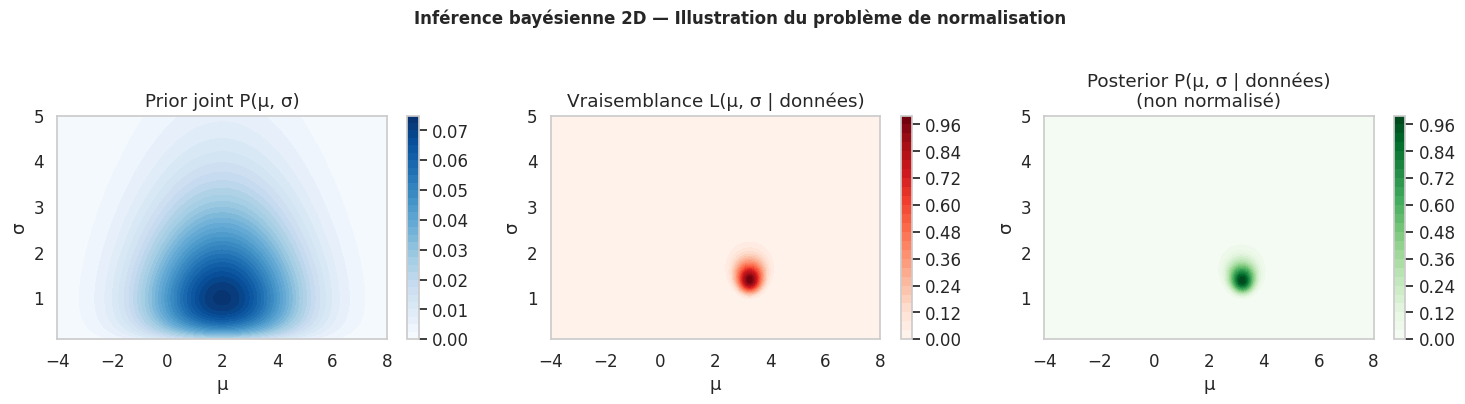
Le chapitre précédent a montré que l’inférence bayésienne requiert de calculer la distribution posterior :
Le problème est le dénominateur : l”evidence \(P(\mathbf{y})\) est une intégrale en dimension \(d\) (le nombre de paramètres). Pour des modèles réalistes avec des priors non-conjugués ou des structures hiérarchiques, cette intégrale est analytiquement intractable et le coût de l’intégration numérique croît exponentiellement avec \(d\).
Les méthodes MCMC (Markov Chain Monte Carlo) contournent ce problème en construisant une chaîne de Markov dont la distribution stationnaire est précisément le posterior souhaité. On n’a pas besoin de normaliser !
Chaînes de Markov : rappels#
Une chaîne de Markov est une suite de variables aléatoires \(\theta^{(1)}, \theta^{(2)}, \ldots\) telle que l’état suivant ne dépend que de l’état courant (propriété de Markov) :
Pour que la chaîne converge vers le posterior cible \(\pi(\theta)\), elle doit être :
Irréductible : tout état est accessible depuis tout autre état
Apériodique : la chaîne ne s’enferme pas dans des cycles
Réversible : condition de bilan détaillé \(\pi(\theta) q(\theta \to \theta') = \pi(\theta') q(\theta' \to \theta)\)
Algorithme de Metropolis-Hastings#
L’algorithme de Metropolis-Hastings (MH) est le fondement de la plupart des méthodes MCMC. Il construit une chaîne en proposant un nouveau point \(\theta^*\) et en l’acceptant ou le rejetant selon un ratio.
Algorithme :
Initialiser \(\theta^{(0)}\) arbitrairement
Pour \(t = 1, 2, \ldots, T\) :
Proposer \(\theta^* \sim q(\theta^* \mid \theta^{(t-1)})\)
Calculer le ratio d’acceptation : \(\alpha = \min\left(1, \frac{\pi(\theta^*) \, q(\theta^{(t-1)} \mid \theta^*)}{\pi(\theta^{(t-1)}) \, q(\theta^* \mid \theta^{(t-1)})}\right)\)
Accepter avec probabilité \(\alpha\) : \(\theta^{(t)} = \theta^*\) ; sinon \(\theta^{(t)} = \theta^{(t-1)}\)
Astuce clé : travail en log
En pratique, le ratio est calculé en log pour éviter les sous-débordements numériques : \(\log \alpha = \log \pi(\theta^*) - \log \pi(\theta^{(t-1)}) + \log q(\theta^{(t-1)}|\theta^*) - \log q(\theta^*|\theta^{(t-1)})\)
Pour une marche aléatoire gaussienne (proposition symétrique), les termes \(q\) s’annulent.
Implémentation complète from scratch#
Exemple : inférence de la moyenne et variance d’une Normale#
def log_prior(mu, log_sigma):
    """Log-prior : mu ~ N(0,10), log(sigma) ~ N(0,1)."""
    lp_mu = norm.logpdf(mu, 0, 10)
    lp_logsigma = norm.logpdf(log_sigma, 0, 1)
    return lp_mu + lp_logsigma

def log_likelihood(data, mu, log_sigma):
    """Log-vraisemblance gaussienne."""
    sigma = np.exp(log_sigma)
    return np.sum(norm.logpdf(data, mu, sigma))

def log_posterior(data, mu, log_sigma):
    """Log-posterior non normalisé."""
    return log_prior(mu, log_sigma) + log_likelihood(data, mu, log_sigma)


def metropolis_hastings(data, n_iter=10000, step_size=0.15, seed=42):
    """
    Metropolis-Hastings avec marche aléatoire gaussienne.
    Paramètres : (mu, log_sigma) pour estimer N(mu, sigma²).
    """
    rng = np.random.default_rng(seed)
    # Initialisation
    theta_curr = np.array([0.0, 0.0])  # (mu, log_sigma)
    lp_curr = log_posterior(data, theta_curr[0], theta_curr[1])

    chain = np.zeros((n_iter, 2))
    accepted = 0

    for t in range(n_iter):
        # Proposition : marche aléatoire gaussienne
        theta_prop = theta_curr + rng.normal(0, step_size, 2)
        lp_prop = log_posterior(data, theta_prop[0], theta_prop[1])

        # Ratio d'acceptation (log-espace)
        log_alpha = lp_prop - lp_curr
        log_u = np.log(rng.uniform())

        if log_u < log_alpha:
            theta_curr = theta_prop
            lp_curr = lp_prop
            accepted += 1

        chain[t] = theta_curr

    taux_accept = accepted / n_iter
    return chain, taux_accept


# Génération des données
np.random.seed(2024)
true_mu, true_sigma = 3.7, 1.4
data_mh = np.random.normal(true_mu, true_sigma, 50)

print(f"Vraies valeurs : μ = {true_mu}, σ = {true_sigma}")
print(f"Statistiques empiriques : ȳ = {data_mh.mean():.3f}, s = {data_mh.std():.3f}")

# Lancer MCMC
chain, taux = metropolis_hastings(data_mh, n_iter=15000, step_size=0.15)
chain_mu = chain[:, 0]
chain_sigma = np.exp(chain[:, 1])  # retour en espace σ

print(f"\nTaux d'acceptation : {taux:.1%}")
print(f"(Idéal : 20-40% pour marche aléatoire)")
Vraies valeurs : μ = 3.7, σ = 1.4
Statistiques empiriques : ȳ = 3.700, s = 1.342
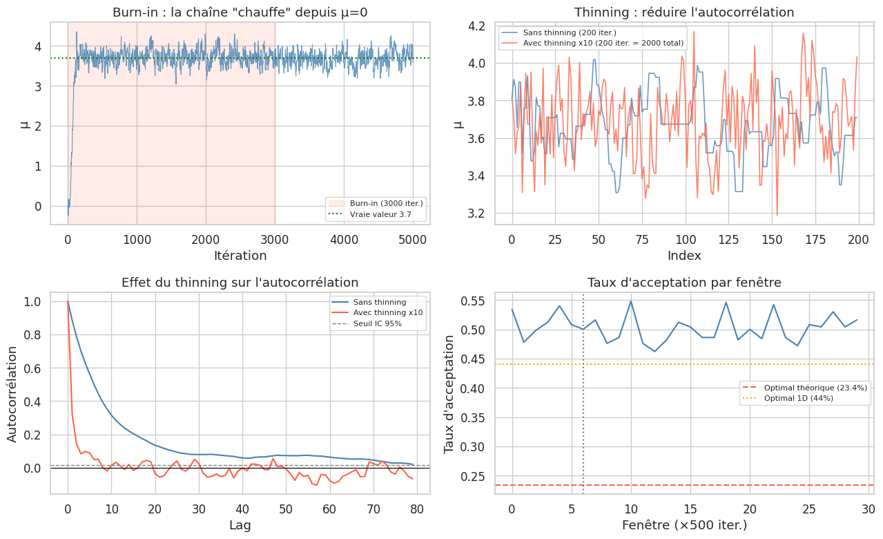
Taux d'acceptation : 50.1%
(Idéal : 20-40% pour marche aléatoire)
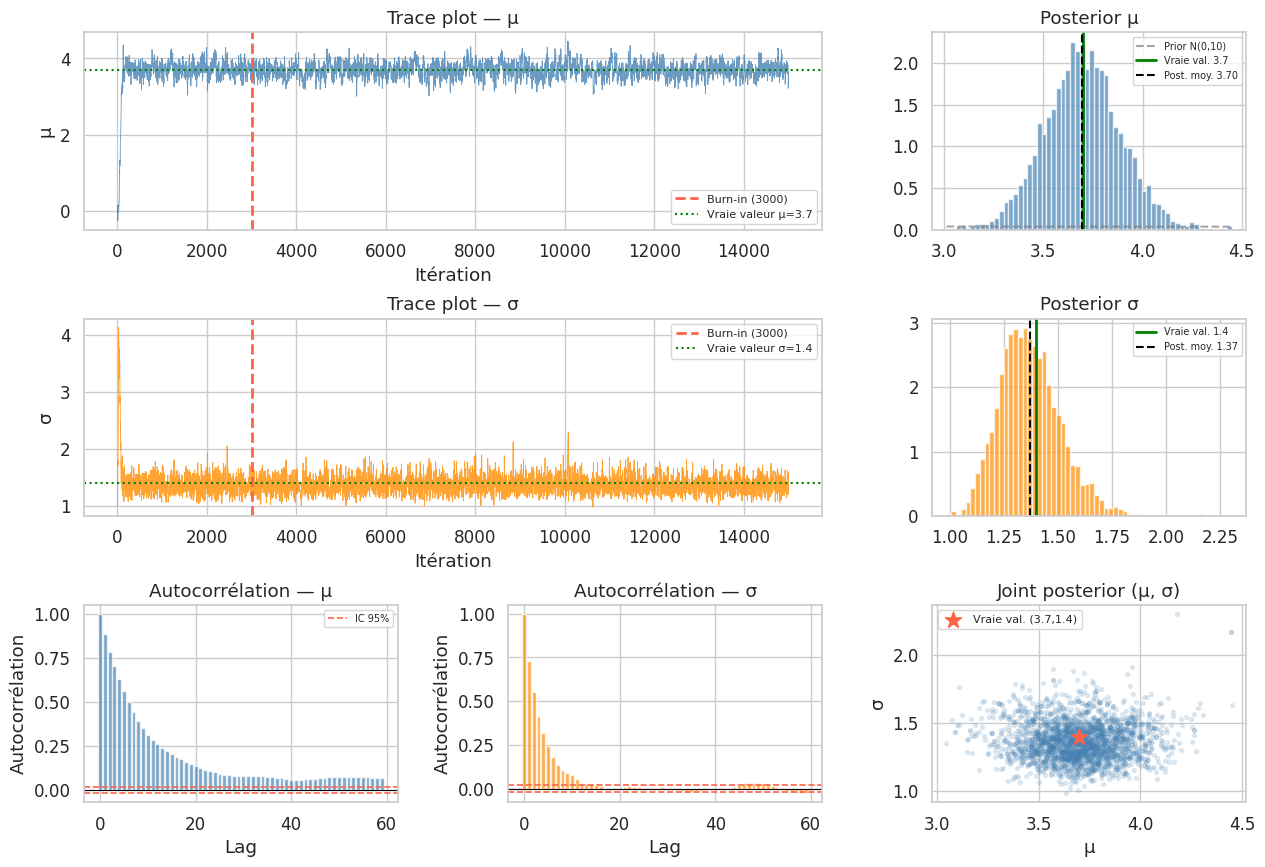
# Résultats après burn-in
burn_in = 3000
chain_mu_post = chain_mu[burn_in:]
chain_sigma_post = chain_sigma[burn_in:]

print("Inférence bayésienne (MCMC) :")
print(f"  μ — Moyenne : {chain_mu_post.mean():.3f}  "
      f"IC 95% : [{np.percentile(chain_mu_post, 2.5):.3f}, {np.percentile(chain_mu_post, 97.5):.3f}]")
print(f"  σ — Moyenne : {chain_sigma_post.mean():.3f}  "
      f"IC 95% : [{np.percentile(chain_sigma_post, 2.5):.3f}, {np.percentile(chain_sigma_post, 97.5):.3f}]")
print(f"\nVraies valeurs : μ = {true_mu}, σ = {true_sigma}")
Inférence bayésienne (MCMC) :
  μ — Moyenne : 3.696  IC 95% : [3.316, 4.081]
  σ — Moyenne : 1.370  IC 95% : [1.125, 1.680]

Vraies valeurs : μ = 3.7, σ = 1.4
Diagnostics MCMC#
Taux d’acceptation#
# Effet de la taille de pas sur le taux d'acceptation
step_sizes = [0.01, 0.05, 0.1, 0.2, 0.5, 1.0, 2.0]
results_steps = []

for step in step_sizes:
    chain_test, taux_test = metropolis_hastings(data_mh, n_iter=5000, step_size=step, seed=1)
    chain_test_post = chain_test[1000:, 0]
    results_steps.append({
        'step_size': step,
        'taux_acceptation': taux_test,
        'ESS_approx': len(chain_test_post) / (1 + 2 * sum(
            [np.corrcoef(chain_test_post[:-l], chain_test_post[l:])[0, 1]
             for l in range(1, min(50, len(chain_test_post)//4))]
        ))
    })

df_steps = pd.DataFrame(results_steps)
print("Effet de la taille de pas :")
print(df_steps.to_string(index=False))
print("\n→ Taux optimal : 20-40% (balance exploration/exploitation)")
Effet de la taille de pas :
 step_size  taux_acceptation  ESS_approx
      0.01            0.9060   40.496172
      0.05            0.8072   74.084814
      0.10            0.6460  201.818813
      0.20            0.3918  419.631522
      0.50            0.1142  209.168353
      1.00            0.0320  105.754691
      2.00            0.0092   49.513696

→ Taux optimal : 20-40% (balance exploration/exploitation)
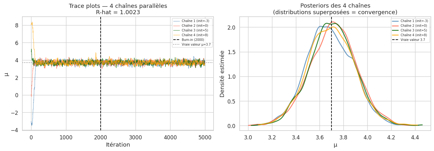
R-hat (Gelman-Rubin)#
Le diagnostic de Gelman-Rubin (\(\hat{R}\)) compare la variance entre plusieurs chaînes et la variance intra-chaîne. Une valeur proche de 1 indique la convergence.
def gelman_rubin(chains):
    """
    Calcule R-hat de Gelman-Rubin pour plusieurs chaînes.
    chains : liste de tableaux 1D de même longueur.
    """
    M = len(chains)    # nombre de chaînes
    N = len(chains[0]) # longueur (après burn-in)

    chain_means = np.array([c.mean() for c in chains])
    overall_mean = chain_means.mean()

    # Variance entre chaînes
    B = N / (M - 1) * np.sum((chain_means - overall_mean) ** 2)
    # Variance intra-chaînes
    W = np.mean([c.var(ddof=1) for c in chains])

    # Variance marginale estimée
    var_hat = (1 - 1/N) * W + B/N
    R_hat = np.sqrt(var_hat / W)
    return R_hat

# Lancer 4 chaînes avec initialisations différentes
chains_mu = []
for seed_i, init_mu in zip([42, 123, 456, 789], [-3, 0, 5, 8]):
    def mh_init(data, init, n_iter=8000, step_size=0.2, seed=42):
        rng = np.random.default_rng(seed)
        theta_curr = np.array([init, 0.0])
        lp_curr = log_posterior(data, theta_curr[0], theta_curr[1])
        chain = np.zeros((n_iter, 2))
        for t in range(n_iter):
            theta_prop = theta_curr + rng.normal(0, step_size, 2)
            lp_prop = log_posterior(data, theta_prop[0], theta_prop[1])
            if np.log(rng.uniform()) < lp_prop - lp_curr:
                theta_curr = theta_prop
                lp_curr = lp_prop
            chain[t] = theta_curr
        return chain

    ch = mh_init(data_mh, init_mu, seed=seed_i)
    chains_mu.append(ch[2000:, 0])  # après burn-in

R_hat = gelman_rubin(chains_mu)
print(f"R-hat (Gelman-Rubin) pour μ : {R_hat:.4f}")
print(f"→ R-hat < 1.01 : convergence excellente")
print(f"→ R-hat < 1.05 : convergence acceptable")
print(f"→ R-hat > 1.1  : chaîne non convergée — augmenter n_iter")
R-hat (Gelman-Rubin) pour μ : 1.0023
→ R-hat < 1.01 : convergence excellente
→ R-hat < 1.05 : convergence acceptable
→ R-hat > 1.1  : chaîne non convergée — augmenter n_iter
Taille effective d’échantillon (ESS)#
L’autocorrélation réduit l’information effective de la chaîne. L’ESS (Effective Sample Size) estime le nombre d’échantillons indépendants équivalents :
def ess(chain, max_lag=200):
    """Calcule l'ESS par la somme des autocorrélations."""
    n = len(chain)
    rho_sum = 0
    for lag in range(1, min(max_lag, n//4)):
        rho = np.corrcoef(chain[:-lag], chain[lag:])[0, 1]
        if rho < 0.05:  # stop quand autocorr négligeable
            break
        rho_sum += rho
    return n / (1 + 2 * rho_sum)

ess_mu = ess(chain_mu_post)
ess_sigma = ess(chain_sigma_post)
n_post = len(chain_mu_post)

print(f"Taille de la chaîne (après burn-in) : {n_post}")
print(f"ESS pour μ : {ess_mu:.0f} ({ess_mu/n_post:.1%} d'efficacité)")
print(f"ESS pour σ : {ess_sigma:.0f} ({ess_sigma/n_post:.1%} d'efficacité)")
print(f"\n→ ESS > 400 est généralement suffisant pour estimer la moyenne et l'IC 95%.")
Taille de la chaîne (après burn-in) : 12000
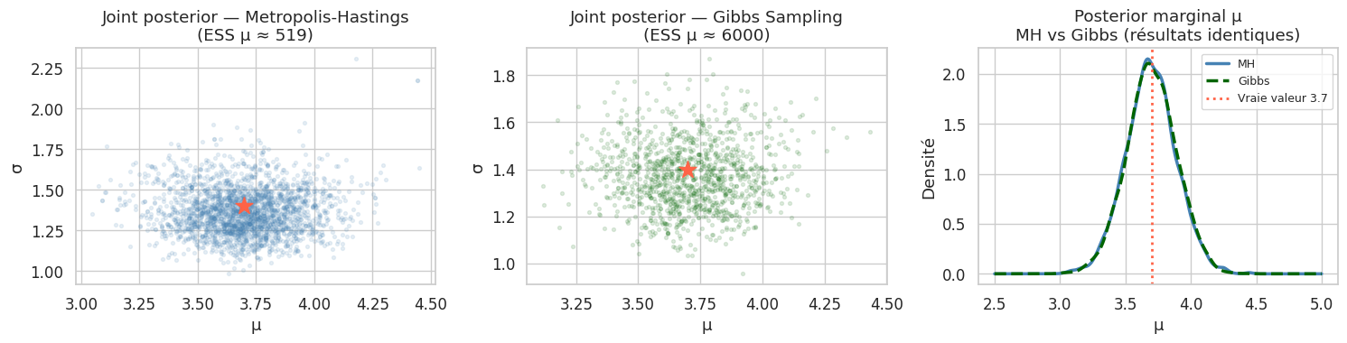
ESS pour μ : 519 (4.3% d'efficacité)
ESS pour σ : 1762 (14.7% d'efficacité)
→ ESS > 400 est généralement suffisant pour estimer la moyenne et l'IC 95%.
Burn-in et thinning#
Gibbs Sampling#
Le Gibbs sampling est un cas particulier de MH où l’on tire chaque paramètre depuis sa distribution conditionnelle complète, en fixant tous les autres. Taux d’acceptation = 100%.
def gibbs_sampler_normal(data, n_iter=8000, seed=42):
    """
    Gibbs sampler pour N(mu, sigma²) avec priors conjugués :
    mu | sigma² ~ N(mu0, tau0²)
    sigma² ~ InvGamma(a0, b0)
    """
    rng = np.random.default_rng(seed)
    n = len(data)
    y_bar = np.mean(data)

    # Hyperparamètres des priors
    mu0, tau0_sq = 0.0, 100.0  # prior sur mu
    a0, b0 = 0.1, 0.1           # prior sur sigma² (quasi non-informatif)

    # Initialisation
    mu_curr = y_bar
    sigma2_curr = np.var(data, ddof=1)

    chain_gibbs = np.zeros((n_iter, 2))

    for t in range(n_iter):
        # 1. Tirer mu | sigma², données
        tau_n_sq = 1 / (1/tau0_sq + n/sigma2_curr)
        mu_n = tau_n_sq * (mu0/tau0_sq + n*y_bar/sigma2_curr)
        mu_curr = rng.normal(mu_n, np.sqrt(tau_n_sq))

        # 2. Tirer sigma² | mu, données
        a_n = a0 + n/2
        b_n = b0 + 0.5 * np.sum((data - mu_curr)**2)
        sigma2_curr = 1 / rng.gamma(a_n, 1/b_n)  # InvGamma via Gamma

        chain_gibbs[t] = [mu_curr, np.sqrt(sigma2_curr)]

    return chain_gibbs

chain_gibbs = gibbs_sampler_normal(data_mh, n_iter=8000)
burn_gibbs = 2000
chain_g_mu = chain_gibbs[burn_gibbs:, 0]
chain_g_sigma = chain_gibbs[burn_gibbs:, 1]

print("Résultats Gibbs Sampling :")
print(f"  μ : {chain_g_mu.mean():.3f}  "
      f"IC 95% : [{np.percentile(chain_g_mu, 2.5):.3f}, {np.percentile(chain_g_mu, 97.5):.3f}]")
print(f"  σ : {chain_g_sigma.mean():.3f}  "
      f"IC 95% : [{np.percentile(chain_g_sigma, 2.5):.3f}, {np.percentile(chain_g_sigma, 97.5):.3f}]")
print(f"\nVraies valeurs : μ = {true_mu}, σ = {true_sigma}")
print(f"ESS μ (Gibbs) : {ess(chain_g_mu):.0f}")
print(f"ESS μ (MH)    : {ess(chain_mu_post):.0f}")
Résultats Gibbs Sampling :
  μ : 3.700  IC 95% : [3.319, 4.073]
  σ : 1.373  IC 95% : [1.127, 1.677]

Vraies valeurs : μ = 3.7, σ = 1.4
ESS μ (Gibbs) : 6000
ESS μ (MH)    : 519
Mentions : PyMC et approximation variationnelle#
PyMC (non installé dans cet environnement)
PyMC est la bibliothèque Python de référence pour la modélisation bayésienne probabiliste. Elle fournit une interface de haut niveau pour spécifier des modèles et utilise des algorithmes avancés comme NUTS (No-U-Turn Sampler, une variante adaptative de HMC).
Exemple de syntaxe PyMC pour le même modèle :
import pymc as pm
with pm.Model() as model:
    mu = pm.Normal('mu', mu=0, sigma=10)
    sigma = pm.HalfNormal('sigma', sigma=1)
    y_obs = pm.Normal('y_obs', mu=mu, sigma=sigma, observed=data)
    trace = pm.sample(2000, tune=1000, chains=4, return_inferencedata=True)
    pm.plot_trace(trace)
Approximation variationnelle (VI)
L”inférence variationnelle remplace l’échantillonnage par un problème d’optimisation : on cherche la distribution \(q(\theta)\) dans une famille paramétrique (ex : Gaussienne) qui minimise la divergence KL avec le posterior. Plus rapide que MCMC mais l’approximation peut être inexacte pour des posteriors complexes ou multimodaux. Implémentée dans PyMC (pm.fit()), TensorFlow Probability, et Pyro.
Résumé#
Points clés — MCMC
Le MCMC permet d’échantillonner des posteriors sans calculer la constante de normalisation.
Metropolis-Hastings : algorithme général, taux d’acceptation cible 20-40% pour une marche aléatoire.
Gibbs Sampling : efficace quand les conditionnelles complètes sont disponibles, taux d’acceptation 100%.
Diagnostics indispensables : trace plots (chaîne mixée ?), R-hat < 1.01 (convergence ?), ESS > 400 (précision ?), autocorrélation (nécessité de thinning ?).
Burn-in : jeter les premières itérations pendant la phase de « chauffe ».
En pratique, utiliser PyMC ou Stan qui implémentent des algorithmes plus efficaces (NUTS/HMC).