Estimation et intervalles de confiance

Contenu

Estimation et intervalles de confiance#

Estimer une quantité à partir d’un échantillon, c’est inévitablement accepter une incertitude. Le point estimé — la valeur calculée sur l’échantillon — n’est qu’une réalisation parmi toutes celles qu’on aurait pu obtenir avec d’autres données. L”intervalle de confiance quantifie cette incertitude de façon opérationnelle. Ce chapitre couvre les méthodes classiques et computationnelles pour construire ces intervalles.

Rappel : estimateur, biais, variance, MSE#

Un estimateur \(\hat{\theta}\) d’un paramètre \(\theta\) est une statistique — une fonction des données — qui approche \(\theta\). Sa qualité se mesure par :

Biais : \(B(\hat{\theta}) = E[\hat{\theta}] - \theta\). Un estimateur sans biais satisfait \(E[\hat{\theta}] = \theta\).
Variance : \(\text{Var}(\hat{\theta})\) — variabilité de l’estimateur d’un échantillon à l’autre.
MSE (Mean Squared Error) : \(\text{MSE}(\hat{\theta}) = \text{Var}(\hat{\theta}) + B(\hat{\theta})^2\) — combine les deux.

Biais vs variance

Il existe un arbitrage fondamental entre biais et variance. La moyenne empirique est sans biais pour \(\mu\) ; l’estimateur shrinkage de James-Stein est biaisé mais peut avoir une MSE plus faible. Pour les démonstrations rigoureuses de ces propriétés, voir le livre Mathématiques, chapitre sur les statistiques mathématiques.

# Illustration : biais de l'estimateur de variance
# s² avec n-1 est sans biais ; avec n est biaisé
sigma_vrai = 5.0
mu_vrai = 10.0
n_obs = 15

n_sim = 10000
var_n = []
var_n1 = []

for _ in range(n_sim):
    x = rng.normal(mu_vrai, sigma_vrai, n_obs)
    var_n.append(np.var(x, ddof=0))   # diviseur n (biaisé)
    var_n1.append(np.var(x, ddof=1))  # diviseur n-1 (sans biais)

print(f"Variance vraie σ²    : {sigma_vrai**2:.4f}")
print(f"E[s²_n]   (ddof=0)  : {np.mean(var_n):.4f}  → biais = {np.mean(var_n)-sigma_vrai**2:.4f}")
print(f"E[s²_n-1] (ddof=1)  : {np.mean(var_n1):.4f}  → biais = {np.mean(var_n1)-sigma_vrai**2:.4f}")

Variance vraie σ²    : 25.0000
E[s²_n]   (ddof=0)  : 23.5351  → biais = -1.4649
E[s²_n-1] (ddof=1)  : 25.2162  → biais = 0.2162

Bootstrap : principe du rééchantillonnage#

Le bootstrap (Efron, 1979) est une méthode computationnelle d’estimation de la distribution d’un estimateur. L’idée centrale : l’échantillon observé est la meilleure approximation disponible de la population. On peut donc rééchantillonner avec remise pour simuler la variabilité.

Algorithme :

À partir de l’échantillon \((x_1, \ldots, x_n)\), tirer \(B\) échantillons bootstrap \((x_1^*, \ldots, x_n^*)\) avec remise.
Calculer l’estimateur \(\hat{\theta}^*_b\) sur chaque échantillon.
La distribution des \(\{\hat{\theta}^*_b\}\) approxime la distribution de \(\hat{\theta}\).

# Bootstrap from scratch
def bootstrap(data, statistic, n_boot=2000, random_state=None):
    """
    Bootstrap non paramétrique.

    Parameters
    ----------
    data : array-like
    statistic : callable — fonction(array) → scalaire
    n_boot : int — nombre de rééchantillons
    random_state : int ou Generator

    Returns
    -------
    array des statistiques bootstrap
    """
    rng_b = np.random.default_rng(random_state)
    data = np.asarray(data)
    n = len(data)
    boots = np.array([
        statistic(rng_b.choice(data, size=n, replace=True))
        for _ in range(n_boot)
    ])
    return boots

# Données : temps de chargement d'une page web (ms)
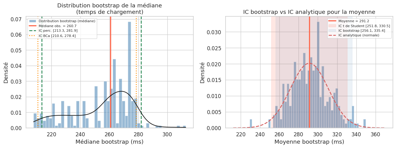
data_web = rng.lognormal(mean=np.log(250), sigma=0.6, size=80)
print(f"n = {len(data_web)}, médiane = {np.median(data_web):.1f} ms")
print(f"Skewness = {stats.skew(data_web):.2f}  → distribution asymétrique")

n = 80, médiane = 260.7 ms
Skewness = 1.85  → distribution asymétrique

Bootstrap percentile#

La méthode la plus simple : les bornes de l’IC sont les quantiles \(\alpha/2\) et \(1-\alpha/2\) de la distribution bootstrap.

Bootstrap BCa (Bias-Corrected and Accelerated)#

Le bootstrap percentile peut être biaisé et sous-optimal. Le BCa (Efron & Tibshirani, 1993) corrige :

Correction de biais \(z_0\) : proportion des valeurs bootstrap inférieures à l’estimateur observé.
Accélération \(a\) : mesure la vitesse de variation de l’écart-type de l’estimateur.

C’est l’IC bootstrap recommandé pour la plupart des applications.

def bootstrap_ic(data, statistic, n_boot=2000, alpha=0.05, methode="bca"):
    """
    IC bootstrap : méthode percentile ou BCa.

    Returns
    -------
    ic_low, ic_high, boots
    """
    boots = bootstrap(data, statistic, n_boot=n_boot, random_state=0)
    theta_hat = statistic(data)

    if methode == "percentile":
        ic_low = np.percentile(boots, 100 * alpha / 2)
        ic_high = np.percentile(boots, 100 * (1 - alpha / 2))

    elif methode == "bca":
        # Correction de biais z0
        z0 = stats.norm.ppf(np.mean(boots < theta_hat) + 1e-10)

        # Accélération a (jackknife)
        n = len(data)
        jk_vals = np.array([statistic(np.delete(data, i)) for i in range(n)])
        jk_mean = jk_vals.mean()
        num = np.sum((jk_mean - jk_vals)**3)
        den = 6 * (np.sum((jk_mean - jk_vals)**2))**1.5
        a = num / den if den != 0 else 0

        # Quantiles ajustés
        z_alpha_lo = stats.norm.ppf(alpha / 2)
        z_alpha_hi = stats.norm.ppf(1 - alpha / 2)

        def adj_quantile(z_in):
            num_q = z0 + z_in
            return stats.norm.cdf(z0 + num_q / (1 - a * num_q))

        q_lo = adj_quantile(z_alpha_lo)
        q_hi = adj_quantile(z_alpha_hi)
        q_lo = np.clip(q_lo, 0.001, 0.999)
        q_hi = np.clip(q_hi, 0.001, 0.999)

        ic_low = np.percentile(boots, 100 * q_lo)
        ic_high = np.percentile(boots, 100 * q_hi)

    return ic_low, ic_high, boots

# Calcul des IC pour la médiane (temps de chargement)
ic_p_low, ic_p_high, boots_perc = bootstrap_ic(data_web, np.median, methode="percentile")
ic_b_low, ic_b_high, boots_bca = bootstrap_ic(data_web, np.median, methode="bca")

print("IC bootstrap pour la médiane des temps de chargement :")
print(f"  Percentile    : [{ic_p_low:.1f}, {ic_p_high:.1f}] ms")
print(f"  BCa           : [{ic_b_low:.1f}, {ic_b_high:.1f}] ms")
print(f"  Médiane obs.  : {np.median(data_web):.1f} ms")

IC bootstrap pour la médiane des temps de chargement :
  Percentile    : [213.3, 281.9] ms
  BCa           : [210.6, 278.4] ms
  Médiane obs.  : 260.7 ms

# Comparaison IC bootstrap pour plusieurs statistiques
statistiques = {
    "Moyenne": np.mean,
    "Médiane": np.median,
    "Écart-type": np.std,
    "P90": lambda x: np.percentile(x, 90),
    "Skewness": stats.skew,
}

print(f"{'Statistique':15s} {'Estimé':>10} {'IC perc. bas':>14} {'IC perc. haut':>14} {'IC BCa bas':>12} {'IC BCa haut':>12}")
print("-" * 82)
for nom, stat in statistiques.items():
    val = stat(data_web)
    ic_p_l, ic_p_h, _ = bootstrap_ic(data_web, stat, methode="percentile")
    ic_b_l, ic_b_h, _ = bootstrap_ic(data_web, stat, methode="bca")
    print(f"{nom:15s} {val:>10.2f} {ic_p_l:>14.2f} {ic_p_h:>14.2f} {ic_b_l:>12.2f} {ic_b_h:>12.2f}")

Statistique         Estimé   IC perc. bas  IC perc. haut   IC BCa bas  IC BCa haut
----------------------------------------------------------------------------------
Moyenne             291.16         255.58         330.93       256.73       332.45

Médiane             260.74         213.28         281.92       210.57       278.43

Écart-type          175.59         126.66         224.11       136.71       244.31

P90                 528.03         402.62         619.36       402.68       623.95

Skewness              1.85           0.79           2.58         1.03         3.10

Show code cell source

Hide code cell source

fig, axes = plt.subplots(1, 2, figsize=(13, 5))

# Distribution bootstrap de la médiane
ax = axes[0]
boots_med = bootstrap(data_web, np.median, n_boot=300, random_state=42)
theta_obs = np.median(data_web)

ax.hist(boots_med, bins=50, density=True, alpha=0.55, color="steelblue",
        label="Distribution bootstrap (médiane)")
ax.axvline(theta_obs, color="tomato", lw=2.5, label=f"Médiane obs. = {theta_obs:.1f}")
ax.axvline(ic_p_low, color="seagreen", lw=2, linestyle="--", label=f"IC perc. [{ic_p_low:.1f}, {ic_p_high:.1f}]")
ax.axvline(ic_p_high, color="seagreen", lw=2, linestyle="--")
ax.axvline(ic_b_low, color="darkorange", lw=2, linestyle=":", label=f"IC BCa [{ic_b_low:.1f}, {ic_b_high:.1f}]")
ax.axvline(ic_b_high, color="darkorange", lw=2, linestyle=":")

kde_x = np.linspace(boots_med.min(), boots_med.max(), 300)
ax.plot(kde_x, stats.gaussian_kde(boots_med)(kde_x), "k-", lw=1.5)
ax.set_xlabel("Médiane bootstrap (ms)")
ax.set_ylabel("Densité")
ax.set_title("Distribution bootstrap de la médiane\n(temps de chargement)")
ax.legend(fontsize=8)

# Comparaison IC bootstrap vs IC analytique pour la moyenne
ax2 = axes[1]
boots_moy = bootstrap(data_web, np.mean, n_boot=300, random_state=42)
mu_obs = np.mean(data_web)
se_obs = np.std(data_web, ddof=1) / np.sqrt(len(data_web))
t_crit = stats.t.ppf(0.975, df=len(data_web)-1)
ic_analytique = (mu_obs - t_crit * se_obs, mu_obs + t_crit * se_obs)
ic_boot_perc = np.percentile(boots_moy, [2.5, 97.5])

ax2.hist(boots_moy, bins=50, density=True, alpha=0.55, color="steelblue")
ax2.axvline(mu_obs, color="tomato", lw=2.5, label=f"Moyenne = {mu_obs:.1f}")
ax2.axvspan(*ic_analytique, alpha=0.15, color="tomato",
            label=f"IC t de Student [{ic_analytique[0]:.1f}, {ic_analytique[1]:.1f}]")
ax2.axvspan(*ic_boot_perc, alpha=0.1, color="steelblue",
            label=f"IC bootstrap [{ic_boot_perc[0]:.1f}, {ic_boot_perc[1]:.1f}]")
# Gaussienne de l'IC analytique
x_norm = np.linspace(mu_obs - 4*se_obs, mu_obs + 4*se_obs, 300)
ax2.plot(x_norm, stats.norm.pdf(x_norm, mu_obs, se_obs), "r--", lw=2,
         label="IC analytique (normale)")
ax2.set_xlabel("Moyenne bootstrap (ms)")
ax2.set_ylabel("Densité")
ax2.set_title("IC bootstrap vs IC analytique pour la moyenne")
ax2.legend(fontsize=8)

plt.tight_layout()
plt.show()

_images/f9c05fc776f0092dee628a71bab4db19bd0ddefc1858b97d28bf6bf502b1504a.png

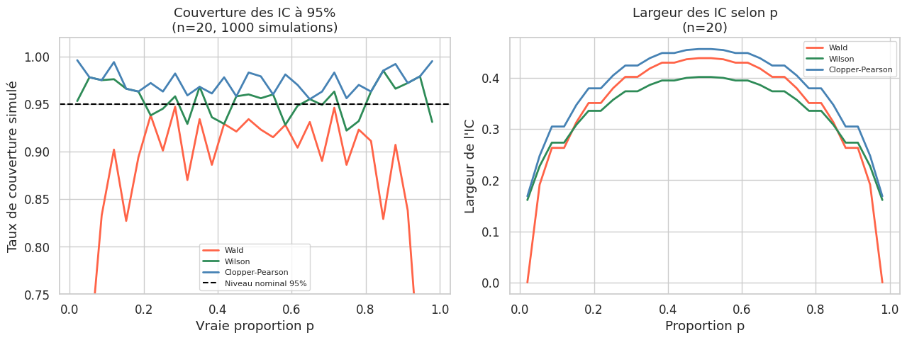
IC pour les proportions#

Estimer une proportion \(p\) à partir de \(k\) succès sur \(n\) essais. Trois méthodes existent, avec des propriétés très différentes.

Approximation normale (Wald)#

\(\hat{p} \pm z_{\alpha/2} \sqrt{\hat{p}(1-\hat{p})/n}\)

Simple mais sous-couvre pour les \(p\) proches de 0 ou 1, ou pour les petits \(n\).

Intervalle de Wilson#

\(\frac{\hat{p} + z^2/(2n) \pm z\sqrt{\hat{p}(1-\hat{p})/n + z^2/(4n^2)}}{1 + z^2/n}\)

Bonne couverture même pour \(p\) extrême ou petit \(n\). C’est la méthode recommandée par défaut.

Intervalle de Clopper-Pearson (exact)#

Basé sur la distribution bêta : \([\text{Beta}(\alpha/2; k, n-k+1), \text{Beta}(1-\alpha/2; k+1, n-k)]\). Garantit une couverture au moins égale à \(1-\alpha\) (conservatif).

def ic_proportion(k, n, alpha=0.05):
    """Trois méthodes d'IC pour une proportion."""
    phat = k / n
    z = stats.norm.ppf(1 - alpha / 2)

    # Wald (normale)
    se_wald = np.sqrt(phat * (1 - phat) / n)
    wald = (phat - z * se_wald, phat + z * se_wald)

    # Wilson
    denom = 1 + z**2 / n
    centre = (phat + z**2 / (2*n)) / denom
    rayon = z * np.sqrt(phat*(1-phat)/n + z**2/(4*n**2)) / denom
    wilson = (centre - rayon, centre + rayon)

    # Clopper-Pearson (exact)
    if k == 0:
        cp_low = 0.0
    else:
        cp_low = stats.beta.ppf(alpha/2, k, n - k + 1)
    if k == n:
        cp_high = 1.0
    else:
        cp_high = stats.beta.ppf(1 - alpha/2, k + 1, n - k)

    return {
        "p_hat": phat,
        "Wald": wald,
        "Wilson": wilson,
        "Clopper-Pearson": (cp_low, cp_high),
    }

# Exemples
print(f"{'Cas':35s} {'Wald':>25} {'Wilson':>25} {'Clopper-Pearson':>25}")
print("-" * 115)
for desc, k, n in [
    ("50/100 (p=0.50, grand n)", 50, 100),
    ("5/10 (p=0.50, petit n)", 5, 10),
    ("95/100 (p=0.95, proche bord)", 95, 100),
    ("1/10 (p=0.10, rare)", 1, 10),
    ("0/20 (zéro succès)", 0, 20),
]:
    res = ic_proportion(k, n)
    wald_s = f"[{res['Wald'][0]:.3f}, {res['Wald'][1]:.3f}]"
    wils_s = f"[{res['Wilson'][0]:.3f}, {res['Wilson'][1]:.3f}]"
    cp_s = f"[{res['Clopper-Pearson'][0]:.3f}, {res['Clopper-Pearson'][1]:.3f}]"
    print(f"{desc:35s} {wald_s:>25} {wils_s:>25} {cp_s:>25}")

Cas                                                      Wald                    Wilson           Clopper-Pearson
-------------------------------------------------------------------------------------------------------------------
50/100 (p=0.50, grand n)                       [0.402, 0.598]            [0.404, 0.596]            [0.398, 0.602]
5/10 (p=0.50, petit n)                         [0.190, 0.810]            [0.237, 0.763]            [0.187, 0.813]
95/100 (p=0.95, proche bord)                   [0.907, 0.993]            [0.888, 0.978]            [0.887, 0.984]
1/10 (p=0.10, rare)                           [-0.086, 0.286]            [0.018, 0.404]            [0.003, 0.445]
0/20 (zéro succès)                             [0.000, 0.000]            [0.000, 0.161]            [0.000, 0.168]

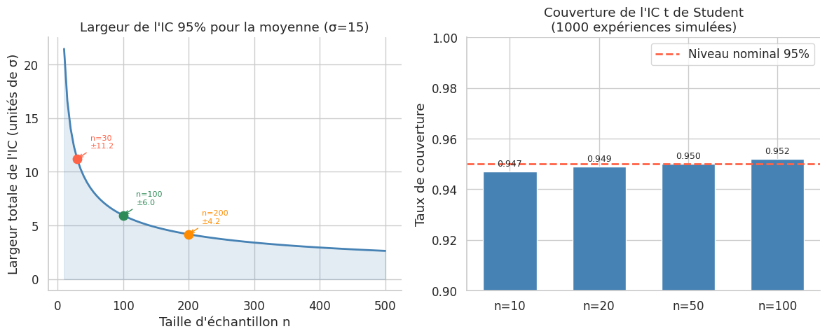
_images/2fe2413a011f3a1dd2fa28f3ba78eb7c20eff769376f9a995c4abfb27a258461.png

Taille d’échantillon et précision de l’IC#

La largeur d’un IC pour la moyenne est \(2 \times t_{\alpha/2} \times \sigma/\sqrt{n}\). Pour réduire la marge d’erreur de moitié, il faut quadrupler \(n\).

def n_necessaire_moyenne(sigma, marge, alpha=0.05, approximation=True):
    """n pour obtenir un IC de ±marge avec écart-type σ connu."""
    z = stats.norm.ppf(1 - alpha/2)
    return int(np.ceil((z * sigma / marge)**2))

def n_necessaire_proportion(marge, p_estime=0.5, alpha=0.05):
    """n pour IC de Wilson de ±marge pour une proportion."""
    z = stats.norm.ppf(1 - alpha/2)
    return int(np.ceil(z**2 * p_estime * (1 - p_estime) / marge**2))

print("Taille d'échantillon nécessaire (IC 95%) :\n")
print("=== Pour une moyenne (σ = 10) ===")
for marge in [5, 2, 1, 0.5]:
    n = n_necessaire_moyenne(sigma=10, marge=marge)
    print(f"  Marge d'erreur ±{marge:4.1f} : n = {n:6d}")

print("\n=== Pour une proportion (p ≈ 0.5, pire cas) ===")
for marge in [0.10, 0.05, 0.03, 0.01]:
    n = n_necessaire_proportion(marge=marge, p_estime=0.5)
    print(f"  Marge d'erreur ±{marge:.2f} : n = {n:6d}")

Taille d'échantillon nécessaire (IC 95%) :

=== Pour une moyenne (σ = 10) ===
  Marge d'erreur ± 5.0 : n =     16
  Marge d'erreur ± 2.0 : n =     97
  Marge d'erreur ± 1.0 : n =    385
  Marge d'erreur ± 0.5 : n =   1537

=== Pour une proportion (p ≈ 0.5, pire cas) ===
  Marge d'erreur ±0.10 : n =     97
  Marge d'erreur ±0.05 : n =    385
  Marge d'erreur ±0.03 : n =   1068
  Marge d'erreur ±0.01 : n =   9604

Show code cell source

Hide code cell source

fig, axes = plt.subplots(1, 2, figsize=(12, 5))

# IC 95% pour la moyenne en fonction de n
sigma_fixe = 15
tailles_n = np.arange(10, 501, 5)
largeurs_ic = [2 * stats.t.ppf(0.975, df=n-1) * sigma_fixe / np.sqrt(n)
               for n in tailles_n]

ax = axes[0]
ax.plot(tailles_n, largeurs_ic, color="steelblue", lw=2)
ax.fill_between(tailles_n, 0, largeurs_ic, alpha=0.15, color="steelblue")
for n_mark, color in [(30, "tomato"), (100, "seagreen"), (200, "darkorange")]:
    larg = 2 * stats.t.ppf(0.975, df=n_mark-1) * sigma_fixe / np.sqrt(n_mark)
    ax.scatter(n_mark, larg, s=80, color=color, zorder=5)
    ax.annotate(f"n={n_mark}\n±{larg:.1f}", xy=(n_mark, larg),
                xytext=(n_mark+20, larg+1), fontsize=8, color=color,
                arrowprops=dict(arrowstyle="->", color=color))
ax.set_xlabel("Taille d'échantillon n")
ax.set_ylabel("Largeur totale de l'IC (unités de σ)")
ax.set_title(f"Largeur de l'IC 95% pour la moyenne (σ={sigma_fixe})")
ax.spines["top"].set_visible(False)
ax.spines["right"].set_visible(False)

# Simulation de couverture des IC à 95% pour la moyenne
n_list = [10, 20, 50, 100]
n_exp = 1000
mu_vrai = 50
sigma_vrai = 10

ax2 = axes[1]
for j, n_t in enumerate(n_list):
    couvertures_n = []
    for _ in range(n_exp):
        x = rng.normal(mu_vrai, sigma_vrai, n_t)
        mu_hat = x.mean()
        se = x.std(ddof=1) / np.sqrt(n_t)
        t_crit = stats.t.ppf(0.975, df=n_t-1)
        ic_lo = mu_hat - t_crit * se
        ic_hi = mu_hat + t_crit * se
        couvertures_n.append(ic_lo <= mu_vrai <= ic_hi)
    couv = np.mean(couvertures_n)
    ax2.bar(j, couv, color="steelblue" if abs(couv - 0.95) < 0.02 else "tomato", width=0.6)
    ax2.text(j, couv + 0.002, f"{couv:.3f}", ha="center", fontsize=9)

ax2.axhline(0.95, color="tomato", lw=2, linestyle="--", label="Niveau nominal 95%")
ax2.set_xticks(range(len(n_list)))
ax2.set_xticklabels([f"n={n}" for n in n_list])
ax2.set_ylabel("Taux de couverture")
ax2.set_ylim(0.90, 1.00)
ax2.set_title(f"Couverture de l'IC t de Student\n({n_exp} expériences simulées)")
ax2.legend()
ax2.spines["top"].set_visible(False)
ax2.spines["right"].set_visible(False)

plt.tight_layout()
plt.show()

_images/d1fa7fd3b37187f6058fde5fcb96c04e409b9ba8a60856259baed389cf9944f1.png

IC pour la différence de moyennes : Welch vs Student#

Comparer deux groupes est l’une des opérations les plus fréquentes. Le test de Student suppose des variances égales ; le test de Welch (recommandé par défaut) ne le suppose pas.

# Deux groupes avec variances différentes
groupe_A = rng.normal(52, 8, 40)
groupe_B = rng.normal(58, 15, 35)

# Student (variance poolée)
diff_obs = groupe_A.mean() - groupe_B.mean()
n_A, n_B = len(groupe_A), len(groupe_B)
s_A, s_B = groupe_A.std(ddof=1), groupe_B.std(ddof=1)

# Variance poolée (Student)
sp2 = ((n_A - 1) * s_A**2 + (n_B - 1) * s_B**2) / (n_A + n_B - 2)
se_student = np.sqrt(sp2 * (1/n_A + 1/n_B))
t_crit_s = stats.t.ppf(0.975, df=n_A + n_B - 2)
ic_student = (diff_obs - t_crit_s * se_student, diff_obs + t_crit_s * se_student)

# Welch (variances distinctes)
se_welch = np.sqrt(s_A**2/n_A + s_B**2/n_B)
df_welch = (s_A**2/n_A + s_B**2/n_B)**2 / (
    (s_A**2/n_A)**2 / (n_A-1) + (s_B**2/n_B)**2 / (n_B-1)
)
t_crit_w = stats.t.ppf(0.975, df=df_welch)
ic_welch = (diff_obs - t_crit_w * se_welch, diff_obs + t_crit_w * se_welch)

# scipy (Welch est la valeur par défaut)
t_stat, p_val = stats.ttest_ind(groupe_A, groupe_B, equal_var=False)

print(f"Groupe A : n={n_A}, μ={groupe_A.mean():.1f}, σ={s_A:.1f}")
print(f"Groupe B : n={n_B}, μ={groupe_B.mean():.1f}, σ={s_B:.1f}")
print(f"Ratio des variances : {(s_B/s_A)**2:.2f}  → variances clairement différentes")
print()
print(f"IC Student 95% (variances égales) : {ic_student[0]:.2f} à {ic_student[1]:.2f}")
print(f"IC Welch 95%   (variances libres) : {ic_welch[0]:.2f} à {ic_welch[1]:.2f}")
print(f"Degrés de liberté Welch : {df_welch:.1f}  (vs {n_A+n_B-2} pour Student)")

Groupe A : n=40, μ=54.1, σ=8.2
Groupe B : n=35, μ=59.1, σ=16.9
Ratio des variances : 4.24  → variances clairement différentes

IC Student 95% (variances égales) : -11.03 à 0.93
IC Welch 95%   (variances libres) : -11.34 à 1.24
Degrés de liberté Welch : 47.7  (vs 73 pour Student)

Welch ou Student ?

Par défaut, utilisez Welch (scipy.stats.ttest_ind(equal_var=False)). Il est robuste lorsque les variances sont égales (très peu de perte de puissance) et correct lorsqu’elles sont différentes. Le test de Student avec variances poolées peut être sévèrement anticonservatif si les variances et les tailles d’échantillon sont toutes deux différentes.

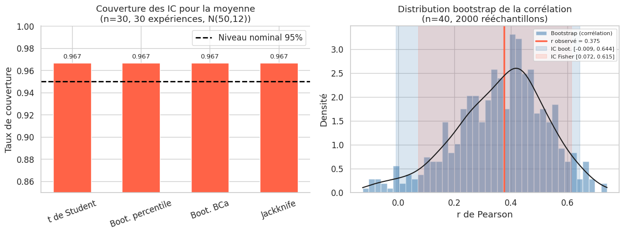
Le Jackknife#

Le jackknife (Quenouille, 1949) est l’ancêtre du bootstrap. Il consiste à recalculer l’estimateur en supprimant tour à tour chaque observation.

\[\hat{\theta}_{-i} = \text{statistique}(x_1, \ldots, x_{i-1}, x_{i+1}, \ldots, x_n)\]

Estimation du biais :

\[\hat{B}_{\text{jk}} = (n-1)(\bar{\hat{\theta}}_{-\cdot} - \hat{\theta})\]

Estimation de la variance :

\[\hat{V}_{\text{jk}} = \frac{n-1}{n} \sum_{i=1}^n (\hat{\theta}_{-i} - \bar{\hat{\theta}}_{-\cdot})^2\]

def jackknife(data, statistic):
    """
    Estimation par jackknife du biais et de la variance.

    Returns
    -------
    dict avec theta_hat, biais_jk, var_jk, se_jk, vals_jk
    """
    data = np.asarray(data)
    n = len(data)
    theta_hat = statistic(data)
    vals_jk = np.array([statistic(np.delete(data, i)) for i in range(n)])
    theta_jk_mean = vals_jk.mean()
    biais = (n - 1) * (theta_jk_mean - theta_hat)
    var_jk = (n-1) / n * np.sum((vals_jk - theta_jk_mean)**2)
    se_jk = np.sqrt(var_jk)
    return {
        "theta_hat": theta_hat,
        "biais_jk": biais,
        "var_jk": var_jk,
        "se_jk": se_jk,
        "theta_corrige": theta_hat - biais,
        "vals_jk": vals_jk,
    }

# Application sur les temps de chargement
print("=== Jackknife sur les temps de chargement ===\n")
for nom, stat in [("Moyenne", np.mean), ("Médiane", np.median),
                   ("Écart-type", np.std), ("Skewness", stats.skew)]:
    res = jackknife(data_web, stat)
    print(f"{nom:12s} : estimé = {res['theta_hat']:8.3f},  "
          f"biais = {res['biais_jk']:8.4f},  "
          f"SE jackknife = {res['se_jk']:8.4f},  "
          f"estimé corrigé = {res['theta_corrige']:8.3f}")

=== Jackknife sur les temps de chargement ===

Moyenne      : estimé =  291.160,  biais =  -0.0000,  SE jackknife =  19.7552,  estimé corrigé =  291.160
Médiane      : estimé =  260.743,  biais =   0.0000,  SE jackknife =  18.7235,  estimé corrigé =  260.743
Écart-type   : estimé =  175.588,  biais =  -3.3029,  SE jackknife =  27.7396,  estimé corrigé =  178.891
Skewness     : estimé =    1.846,  biais =  -0.2882,  SE jackknife =   0.7214,  estimé corrigé =    2.134

Show code cell source

Hide code cell source

# Comparaison bootstrap vs jackknife : simulation de couverture (1000 expériences)
fig, axes = plt.subplots(1, 2, figsize=(13, 5))

n_experience = 30
mu_vrai = 50
sigma_vrai = 12
n_obs = 30

couv_t = 0
couv_boot_perc = 0
couv_boot_bca = 0
couv_jk = 0

for _ in range(n_experience):
    x = rng.normal(mu_vrai, sigma_vrai, n_obs)
    mu_hat = x.mean()
    se = x.std(ddof=1) / np.sqrt(n_obs)
    t_c = stats.t.ppf(0.975, df=n_obs-1)

    # IC t
    if mu_hat - t_c*se <= mu_vrai <= mu_hat + t_c*se:
        couv_t += 1

    # IC bootstrap percentile
    b_p_l, b_p_h, _ = bootstrap_ic(x, np.mean, n_boot=200, methode="percentile")
    if b_p_l <= mu_vrai <= b_p_h:
        couv_boot_perc += 1

    # IC bootstrap BCa
    b_b_l, b_b_h, _ = bootstrap_ic(x, np.mean, n_boot=200, methode="bca")
    if b_b_l <= mu_vrai <= b_b_h:
        couv_boot_bca += 1

    # IC jackknife
    res_jk = jackknife(x, np.mean)
    z_jk = stats.norm.ppf(0.975)
    if mu_hat - z_jk*res_jk["se_jk"] <= mu_vrai <= mu_hat + z_jk*res_jk["se_jk"]:
        couv_jk += 1

couvertures_finales = {
    "t de Student": couv_t / n_experience,
    "Boot. percentile": couv_boot_perc / n_experience,
    "Boot. BCa": couv_boot_bca / n_experience,
    "Jackknife": couv_jk / n_experience,
}

# Graphique de couverture
ax = axes[0]
noms_m = list(couvertures_finales.keys())
covs = list(couvertures_finales.values())
colors = ["seagreen" if abs(c - 0.95) < 0.015 else "tomato" for c in covs]
bars = ax.bar(noms_m, covs, color=colors, width=0.55)
ax.axhline(0.95, color="black", lw=2, linestyle="--", label="Niveau nominal 95%")
ax.set_ylim(0.85, 1.00)
for bar, c in zip(bars, covs):
    ax.text(bar.get_x() + bar.get_width()/2, c + 0.003, f"{c:.3f}",
            ha="center", va="bottom", fontsize=9.5)
ax.set_ylabel("Taux de couverture")
ax.set_title(f"Couverture des IC pour la moyenne\n(n={n_obs}, {n_experience} expériences, N(50,12))")
ax.legend()
ax.tick_params(axis="x", rotation=20)
ax.spines["top"].set_visible(False)
ax.spines["right"].set_visible(False)

# Illustration jackknife vs bootstrap pour une statistique difficile
ax2 = axes[1]
# Corrélation : statistique pour laquelle jackknife et bootstrap diffèrent
x_corr = rng.normal(0, 1, 40)
y_corr = 0.5 * x_corr + rng.normal(0, 0.8, 40)
data_corr = np.column_stack([x_corr, y_corr])

def pearson_r(data_2d):
    return stats.pearsonr(data_2d[:, 0], data_2d[:, 1])[0]

r_obs = pearson_r(data_corr)

# Bootstrap
boots_r = []
for _ in range(500):
    idx = rng.integers(0, len(data_corr), size=len(data_corr))
    boots_r.append(pearson_r(data_corr[idx]))
boots_r = np.array(boots_r)
ic_r_boot = np.percentile(boots_r, [2.5, 97.5])

# IC de Fisher (transformation de Fisher)
z_r = np.arctanh(r_obs)
se_z = 1 / np.sqrt(len(data_corr) - 3)
ic_r_fish = (
    np.tanh(z_r - 1.96 * se_z),
    np.tanh(z_r + 1.96 * se_z)
)

ax2.hist(boots_r, bins=40, density=True, alpha=0.55, color="steelblue",
         label="Bootstrap (corrélation)")
ax2.axvline(r_obs, color="tomato", lw=2.5, label=f"r observé = {r_obs:.3f}")
ax2.axvspan(*ic_r_boot, alpha=0.2, color="steelblue",
            label=f"IC boot. [{ic_r_boot[0]:.3f}, {ic_r_boot[1]:.3f}]")
ax2.axvspan(*ic_r_fish, alpha=0.15, color="tomato",
            label=f"IC Fisher [{ic_r_fish[0]:.3f}, {ic_r_fish[1]:.3f}]")
x_kde = np.linspace(boots_r.min(), boots_r.max(), 300)
ax2.plot(x_kde, stats.gaussian_kde(boots_r)(x_kde), "k-", lw=1.5)
ax2.set_xlabel("r de Pearson")
ax2.set_ylabel("Densité")
ax2.set_title("Distribution bootstrap de la corrélation\n(n=40, 2000 rééchantillons)")
ax2.legend(fontsize=8)

plt.tight_layout()
plt.show()

_images/efeaee5ce2917ea32c5d001105515153eaffd84706d4440dbb48085d66e6ede0.png

Récapitulatif des méthodes#

                                                        Hypothèses                     Quand l'utiliser                                         Limites
Méthode                                                                                                                                                
IC t de Student (moyenne)                     Normalité ou grand n  Moyenne, n ≥ 30 ou données normales              Sensible aux outliers pour petit n
IC Welch (diff. de moyennes)       Indépendance, normalité approx.    Comparaison deux groupes (défaut)                                    Idem Student
IC Wilson (proportion)               Indépendance des observations           Proportions, usage général              Léger sous-couvrement aux extrêmes
IC Clopper-Pearson (proportion)      Indépendance des observations  Proportions, garantie de couverture                    Conservatif (IC trop larges)
Bootstrap percentile                              IID, n suffisant   Toute statistique, données simples              Biaisé si distribution asymétrique
Bootstrap BCa                               IID, n ≥ 20 recommandé         Toute statistique, IC précis                       Coûteux, jackknife pour a
Jackknife                        IID, régularité de la statistique         Estimation du biais, petit n  Inexact pour statistiques non-lisses (médiane)

L’intervalle de confiance est une réponse calibrée à une question fondamentale : « quelle est notre incertitude sur ce que les données nous disent ? » Sa construction, qu’elle soit analytique ou computationnelle, repose toujours sur le même principe — simuler (analytiquement ou par rééchantillonnage) ce qui se passerait si on répétait l’expérience. Comprendre ce principe, c’est comprendre la logique entière de l’inférence statistique fréquentiste.