Diagnostic et monitoring réseau#
Le diagnostic réseau est l’art de comprendre pourquoi une connexion est lente, instable ou interrompue. Le monitoring consiste à observer en continu l’état du réseau pour détecter les anomalies avant qu’elles n’impactent les utilisateurs. Dans ce chapitre, nous couvrons les outils classiques (ping, traceroute, netstat), la lecture des métriques système Linux, et les architectures de monitoring modernes avec Prometheus et Grafana.
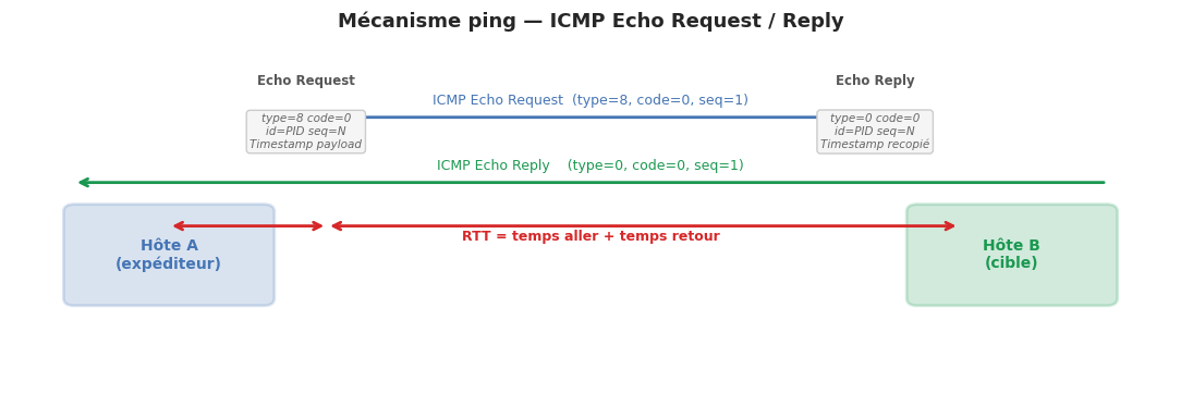
ping — ICMP Echo Request/Reply#
ping est l’outil de diagnostic réseau le plus fondamental. Il envoie des messages ICMP Echo Request et mesure le temps de réponse (RTT — Round Trip Time).
Fonctionnement ICMP#
fig, ax = plt.subplots(figsize=(11, 4))
ax.set_xlim(0, 11)
ax.set_ylim(0, 5)
ax.axis('off')
ax.set_title("Mécanisme ping — ICMP Echo Request / Reply", fontsize=13, fontweight='bold', pad=12)

# Entités
for x, label, col in [(1.5, "Hôte A\n(expéditeur)", '#4575b4'), (9.5, "Hôte B\n(cible)", '#1a9850')]:
    ax.add_patch(mpatches.FancyBboxPatch((x-0.9, 1.5), 1.8, 1.2,
                 boxstyle="round,pad=0.1", facecolor=col, alpha=0.2,
                 edgecolor=col, linewidth=2))
    ax.text(x, 2.1, label, ha='center', va='center', fontsize=10, fontweight='bold', color=col)

# Flèches
for y, texte, x1, x2, col in [
    (4.0, "ICMP Echo Request  (type=8, code=0, seq=1)", 1.5, 9.5, '#4575b4'),
    (3.1, "ICMP Echo Reply    (type=0, code=0, seq=1)", 9.5, 1.5, '#1a9850'),
    (2.8, "← RTT = t₂ − t₁ →", 1.5, 9.5, '#d62728'),
]:
    if '←' not in texte:
        ax.annotate("", xy=(x2-0.9, y), xytext=(x1+0.9, y),
                    arrowprops=dict(arrowstyle='->', color=col, lw=2))
        ax.text((x1+x2)/2, y+0.18, texte, ha='center', fontsize=9, color=col)
    else:
        ax.annotate("", xy=(3.0, 2.5), xytext=(1.5, 2.5),
                    arrowprops=dict(arrowstyle='<->', color='#d62728', lw=2))
        ax.annotate("", xy=(9.0, 2.5), xytext=(3.0, 2.5),
                    arrowprops=dict(arrowstyle='<->', color='#d62728', lw=2))
        ax.text(5.5, 2.3, "RTT = temps aller + temps retour", ha='center',
                fontsize=9, color='#d62728', fontweight='bold')

# Champs ICMP
for x, titre, champs in [
    (2.8, "Echo Request", "type=8 code=0\nid=PID seq=N\nTimestamp payload"),
    (8.2, "Echo Reply",   "type=0 code=0\nid=PID seq=N\nTimestamp recopié"),
]:
    ax.text(x, 4.5, titre, ha='center', va='center', fontsize=8.5,
            fontweight='bold', color='#555555')
    ax.text(x, 3.8, champs, ha='center', va='center', fontsize=7.5,
            color='#666666', style='italic',
            bbox=dict(boxstyle='round,pad=0.3', facecolor='#f5f5f5', edgecolor='#cccccc'))

plt.tight_layout()
plt.savefig('_static/ping_icmp.png', dpi=100, bbox_inches='tight')
plt.show()
Interprétation de la sortie ping#
PING google.com (142.250.74.206) 56(84) bytes of data.
64 bytes from 142.250.74.206: icmp_seq=1 ttl=118 time=11.3 ms
64 bytes from 142.250.74.206: icmp_seq=2 ttl=118 time=10.9 ms
64 bytes from 142.250.74.206: icmp_seq=3 ttl=118 time=11.1 ms

--- google.com ping statistics ---
3 packets transmitted, 3 received, 0% packet loss
round-trip min/avg/max/mdev = 10.9/11.1/11.3/0.163 ms
ttl=118 : le paquet a traversé 64−118 = … non — le TTL de départ est souvent 128 (Windows) ou 64/255 (Linux). Ici TTL=118 depuis un départ de 128 → 10 sauts.
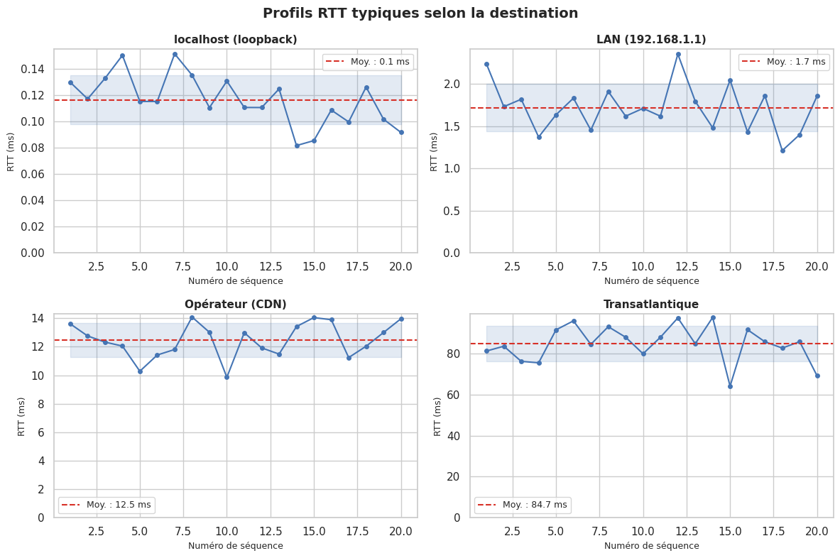
time : RTT en millisecondes. < 1 ms = local ; 1–20 ms = réseau local/national ; > 100 ms = intercontinental ou congestion.
mdev : déviation moyenne (jitter). Un mdev élevé indique une instabilité réseau.
# Simulation de mesures RTT avec ping (sans socket raw — mesure TCP comme substitut pédagogique)

def mesurer_rtt_tcp(hôte: str, port: int = 80, n: int = 5, timeout: float = 2.0) -> list[float]:
    """
    Mesure le RTT en établissant une connexion TCP (non un ping ICMP).
    Pédagogique : illustre le concept de RTT sans droits root.
    """
    rtts = []
    for _ in range(n):
        try:
            t0 = time.perf_counter()
            sock = socket.socket(socket.AF_INET, socket.SOCK_STREAM)
            sock.settimeout(timeout)
            sock.connect((hôte, port))
            t1 = time.perf_counter()
            sock.close()
            rtts.append((t1 - t0) * 1000)  # en ms
        except Exception:
            rtts.append(None)
    return rtts

# Données simulées représentatives (évite dépendance réseau externe)
np.random.seed(42)

cibles = {
    'localhost (loopback)':  np.random.normal(0.12, 0.02, 20),
    'LAN (192.168.1.1)':     np.random.normal(1.8,  0.3,  20),
    'Opérateur (CDN)':       np.random.normal(12.5, 1.5,  20),
    'Transatlantique':       np.random.normal(85,   8,    20),
}

fig, axes = plt.subplots(2, 2, figsize=(12, 8))
fig.suptitle("Profils RTT typiques selon la destination", fontsize=14, fontweight='bold')

for (titre, rtts), ax in zip(cibles.items(), axes.flat):
    indices = range(1, len(rtts)+1)
    ax.plot(indices, rtts, 'o-', color='#4575b4', linewidth=1.5, markersize=4)
    ax.axhline(np.mean(rtts), color='#d73027', linestyle='--', linewidth=1.5,
               label=f"Moy. : {np.mean(rtts):.1f} ms")
    ax.fill_between(indices, np.mean(rtts)-np.std(rtts), np.mean(rtts)+np.std(rtts),
                    alpha=0.15, color='#4575b4')
    ax.set_title(titre, fontsize=11, fontweight='bold')
    ax.set_xlabel("Numéro de séquence", fontsize=9)
    ax.set_ylabel("RTT (ms)", fontsize=9)
    ax.legend(fontsize=9)
    ax.set_ylim(0, None)

plt.tight_layout()
plt.savefig('_static/rtt_profiles.png', dpi=100, bbox_inches='tight')
plt.show()
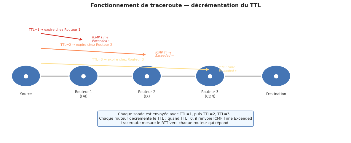
traceroute — cartographier le chemin réseau#
traceroute (Unix) ou tracert (Windows) révèle la liste des routeurs intermédiaires entre la source et la destination, ainsi que le RTT vers chacun d’eux.
Mécanisme : exploitation du TTL#
fig, ax = plt.subplots(figsize=(12, 5))
ax.set_xlim(0, 12)
ax.set_ylim(0, 6)
ax.axis('off')
ax.set_title("Fonctionnement de traceroute — décrémentation du TTL", fontsize=13, fontweight='bold', pad=12)

nœuds = [
    (0.8, 3, "Source"),
    (2.8, 3, "Routeur 1\n(FAI)"),
    (5.0, 3, "Routeur 2\n(IX)"),
    (7.2, 3, "Routeur 3\n(CDN)"),
    (9.5, 3, "Destination"),
]
for x, y, label in nœuds:
    ax.add_patch(plt.Circle((x, y), 0.5, facecolor='#4575b4', edgecolor='white', linewidth=2))
    ax.text(x, y, "●", ha='center', va='center', fontsize=14, color='white')
    ax.text(x, y - 0.85, label, ha='center', va='center', fontsize=8.5, color='#333333')

# Flèches de connexion
for i in range(len(nœuds)-1):
    x1, x2 = nœuds[i][0]+0.5, nœuds[i+1][0]-0.5
    ax.annotate("", xy=(x2, 3), xytext=(x1, 3),
                arrowprops=dict(arrowstyle='-', color='#666666', lw=2))

# Paquets avec TTL décroissant
sonde_y = [5.0, 4.3, 3.6]
ttls    = [1, 2, 3]
couleurs_ttl = ['#d73027', '#fc8d59', '#fee090']

for (ttl, y, col) in zip(ttls, sonde_y, couleurs_ttl):
    x_dest = nœuds[ttl][0]
    ax.annotate("", xy=(x_dest, y - 0.3), xytext=(nœuds[0][0] + 0.5, y),
                arrowprops=dict(arrowstyle='->', color=col, lw=1.8))
    ax.text((nœuds[0][0] + x_dest)/2, y + 0.12,
            f"TTL={ttl} → expire chez Routeur {ttl}", ha='center',
            fontsize=8, color=col)
    ax.text(x_dest + 0.3, y - 0.4,
            "ICMP Time\nExceeded ←", ha='left', fontsize=7.5, color=col, style='italic')

ax.text(6, 1.0,
        "Chaque sonde est envoyée avec TTL=1, puis TTL=2, TTL=3…\n"
        "Chaque routeur décrémente le TTL ; quand TTL=0, il renvoie ICMP Time Exceeded\n"
        "traceroute mesure le RTT vers chaque routeur qui répond.",
        ha='center', va='center', fontsize=9, color='#333333',
        bbox=dict(boxstyle='round,pad=0.4', facecolor='#f0f8ff', edgecolor='#4575b4'))

plt.tight_layout()
plt.savefig('_static/traceroute_mechanism.png', dpi=100, bbox_inches='tight')
plt.show()
# Commande traceroute classique (Linux)
traceroute -n google.com

# Avec UDP (défaut Linux) ou ICMP (-I) ou TCP (-T)
traceroute -I -n 8.8.8.8        # sondes ICMP
traceroute -T -p 443 -n 8.8.8.8 # sondes TCP port 443

# tracepath : traceroute sans droits root
tracepath -n google.com

# Affichage typique :
# 1  192.168.1.1   1.234 ms  1.198 ms  1.201 ms
# 2  10.0.0.1      3.412 ms  3.389 ms  3.401 ms
# 3  *  *  *           ← routeur qui ne répond pas ICMP
# 4  74.125.52.24  11.24 ms  11.19 ms  11.22 ms
Étoiles dans traceroute
Les lignes * * * indiquent que le routeur intermédiaire ne répond pas aux sondes ICMP (filtrage par firewall) ou que les paquets ICMP Time Exceeded sont perdus. Cela n’implique pas que le trafic applicatif est bloqué à cet endroit.
netstat et ss#
netstat et son successeur ss (plus rapide, plus complet) affichent l’état des connexions réseau du système.
# Afficher toutes les connexions TCP actives (ss)
ss -tnp

# Afficher les ports en écoute (TCP et UDP)
ss -tlnup

# Afficher les statistiques réseau
ss -s

# Connexions établies vers l'extérieur
ss -tn state established

# Filtrer par port
ss -tn dst :443

# Afficher le processus associé à chaque connexion (root requis)
ss -tnp | grep ESTABLISHED

# Équivalents netstat (moins performant sur les grands systèmes)
netstat -tnp        # connexions TCP avec PID
netstat -rn         # table de routage
netstat -i          # statistiques des interfaces
netstat -s          # statistiques par protocole
Exemple de sortie ss -tnp :
State    Recv-Q Send-Q  Local Address:Port  Peer Address:Port  Process
ESTAB    0      0       192.168.1.10:52341  142.250.74.206:443 ("chromium",pid=1234)
ESTAB    0      0       192.168.1.10:52342  93.184.216.34:443  ("curl",pid=5678)
LISTEN   0      128     0.0.0.0:22          0.0.0.0:*         ("sshd",pid=890)
LISTEN   0      128     127.0.0.1:5432      0.0.0.0:*         ("postgres",pid=456)
nmap — scan et inventaire réseau#
# Découverte d'hôtes actifs (ping scan — sans scan de ports)
nmap -sn 192.168.1.0/24

# Scan des 1000 ports TCP les plus courants
nmap -sT 192.168.1.10

# Détection de version des services
nmap -sV 192.168.1.10

# Détection du système d'exploitation
nmap -O 192.168.1.10

# Scan rapide avec détection OS et version
nmap -A 192.168.1.10

# Scripts NSE de sécurité
nmap --script vuln 192.168.1.10
nmap --script ssl-cert,ssl-enum-ciphers -p 443 192.168.1.10

# Scan discret (SYN, pas de résolution DNS, timing paranoïde)
nmap -sS -n -T1 192.168.1.0/24
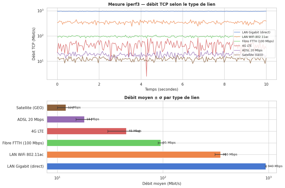
iperf3 — mesure de bande passante#
iperf3 mesure le débit réel entre deux machines en injectant du trafic TCP ou UDP.
# Sur la machine serveur
iperf3 -s

# Sur la machine client — test TCP (10 secondes)
iperf3 -c 192.168.1.1 -t 10

# Test UDP avec débit cible de 100 Mbps
iperf3 -c 192.168.1.1 -u -b 100M

# Fenêtre TCP explicite (pour tester des liens à haute latence)
iperf3 -c 192.168.1.1 -w 4M

# Test bidirectionnel simultané
iperf3 -c 192.168.1.1 --bidir

# JSON output pour traitement automatisé
iperf3 -c 192.168.1.1 -J > résultats.json
# Simulation de résultats iperf3 — débit TCP sur différents liens

np.random.seed(0)

liens = {
    'LAN Gigabit (direct)':       (940,  8,  'fibre_locale'),
    'LAN WiFi 802.11ac':          (350,  40, 'wifi'),
    'Fibre FTTH (100 Mbps)':      (95,   5,  'fibre_ftth'),
    '4G LTE':                     (45,   15, '4g'),
    'ADSL 20 Mbps':               (18,   3,  'adsl'),
    'Satellite (GEO)':            (12,   2,  'sat'),
}

fig, axes = plt.subplots(2, 1, figsize=(12, 8))

# Débit au fil du temps pour chaque lien
ax = axes[0]
t = np.linspace(0, 10, 200)
for (nom, (débit, sigma, _)), col in zip(liens.items(), sns.color_palette('muted', len(liens))):
    bruit = np.random.normal(débit, sigma, len(t))
    bruit = np.clip(bruit, 0, None)
    ax.plot(t, bruit, linewidth=1.5, label=nom, color=col, alpha=0.8)

ax.set_xlabel("Temps (secondes)", fontsize=11)
ax.set_ylabel("Débit TCP (Mbit/s)", fontsize=11)
ax.set_title("Mesure iperf3 — débit TCP selon le type de lien", fontsize=12, fontweight='bold')
ax.legend(fontsize=8.5, loc='right')
ax.set_yscale('log')

# Barres comparatives débit moyen ± σ
ax2 = axes[1]
noms   = list(liens.keys())
débits = [v[0] for v in liens.values()]
sigmas = [v[1] for v in liens.values()]
cols   = sns.color_palette('muted', len(noms))

bars = ax2.barh(noms, débits, xerr=sigmas, color=cols, edgecolor='white',
                height=0.55, capsize=4, error_kw=dict(elinewidth=1.5, ecolor='#333333'))
ax2.set_xlabel("Débit moyen (Mbit/s)", fontsize=11)
ax2.set_title("Débit moyen ± σ par type de lien", fontsize=12, fontweight='bold')
ax2.set_xscale('log')
for bar, val in zip(bars, débits):
    ax2.text(val * 1.05, bar.get_y() + bar.get_height()/2,
             f"{val} Mbps", va='center', fontsize=9)

plt.tight_layout()
plt.savefig('_static/iperf3_results.png', dpi=100, bbox_inches='tight')
plt.show()
Métriques réseau Linux : /proc/net/#
Linux expose des statistiques réseau détaillées via le pseudo-système de fichiers /proc/net/.
import os
import re

def lire_proc_net_dev() -> pd.DataFrame:
    """
    Lit /proc/net/dev et retourne un DataFrame avec les statistiques
    d'octets, paquets, erreurs pour chaque interface.
    Retourne des données simulées si le fichier n'est pas disponible.
    """
    chemin = '/proc/net/dev'
    if os.path.exists(chemin):
        with open(chemin) as f:
            lignes = f.readlines()
        données = []
        for ligne in lignes[2:]:
            # Interface: rx_bytes rx_pkts rx_errs rx_drop ... tx_bytes tx_pkts ...
            champs = ligne.split()
            if len(champs) >= 10:
                iface = champs[0].rstrip(':')
                données.append({
                    'interface':  iface,
                    'rx_octets':  int(champs[1]),
                    'rx_paquets': int(champs[2]),
                    'rx_erreurs': int(champs[3]),
                    'rx_drops':   int(champs[4]),
                    'tx_octets':  int(champs[9]),
                    'tx_paquets': int(champs[10]),
                    'tx_erreurs': int(champs[11]),
                    'tx_drops':   int(champs[12]),
                })
        return pd.DataFrame(données)
    else:
        # Données simulées pour la démo hors Linux
        return pd.DataFrame([
            {'interface':'lo',   'rx_octets':1_234_567, 'rx_paquets':9876, 'rx_erreurs':0, 'rx_drops':0,
             'tx_octets':1_234_567, 'tx_paquets':9876, 'tx_erreurs':0, 'tx_drops':0},
            {'interface':'eth0', 'rx_octets':987_654_321, 'rx_paquets':823456, 'rx_erreurs':12, 'rx_drops':3,
             'tx_octets':456_789_012, 'tx_paquets':512345, 'tx_erreurs':0, 'tx_drops':0},
            {'interface':'wlan0','rx_octets':234_567_890, 'rx_paquets':189234, 'rx_erreurs':45, 'rx_drops':8,
             'tx_octets':123_456_789, 'tx_paquets':98765,  'tx_erreurs':2, 'tx_drops':1},
        ])

df_net = lire_proc_net_dev()
print("Statistiques /proc/net/dev :")
print(df_net.to_string(index=False))

# Calcul du taux d'erreurs
df_net['taux_erreurs_rx_%'] = (
    (df_net['rx_erreurs'] + df_net['rx_drops']) /
    df_net['rx_paquets'].clip(1) * 100
).round(4)
print("\nTaux d'erreurs RX :")
print(df_net[['interface', 'rx_paquets', 'rx_erreurs', 'rx_drops', 'taux_erreurs_rx_%']].to_string(index=False))
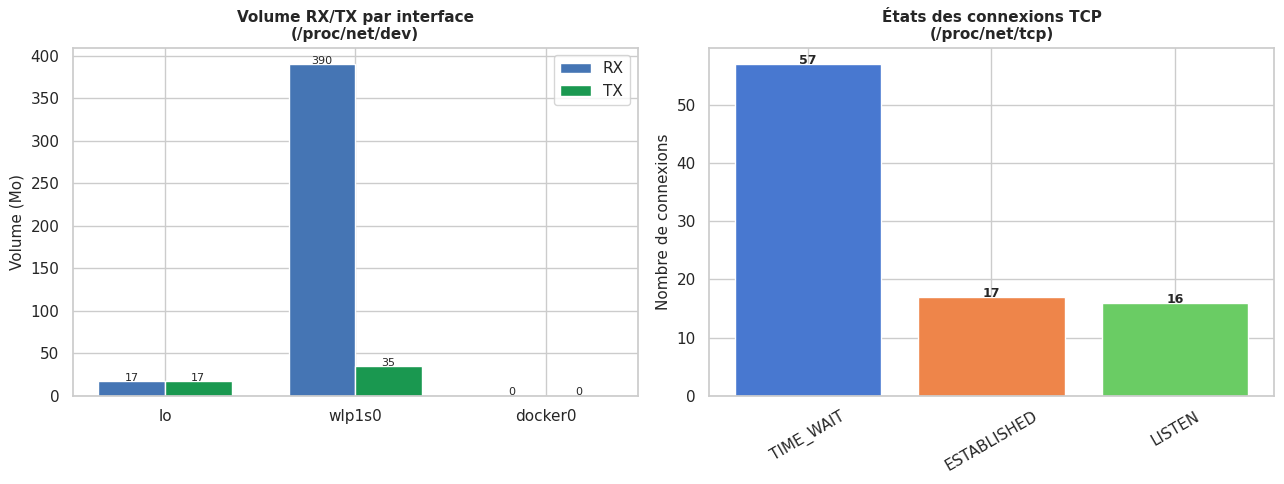
Statistiques /proc/net/dev :
interface  rx_octets  rx_paquets  rx_erreurs  rx_drops  tx_octets  tx_paquets  tx_erreurs  tx_drops
       lo   17133849       15618           0         0   17133849       15618           0         0
   wlp1s0  389949425      354945           0         0   34813168      104458           0         0
  docker0          0           0           0         0          0           0           0        32

Taux d'erreurs RX :
interface  rx_paquets  rx_erreurs  rx_drops  taux_erreurs_rx_%
       lo       15618           0         0                0.0
   wlp1s0      354945           0         0                0.0
  docker0           0           0         0                0.0
def lire_proc_net_tcp() -> pd.DataFrame:
    """
    Lit /proc/net/tcp (connexions TCP).
    Retourne des données simulées si indisponible.
    """
    chemin = '/proc/net/tcp'

    états_tcp = {
        '01':'ESTABLISHED', '02':'SYN_SENT', '03':'SYN_RECV',
        '04':'FIN_WAIT1',   '05':'FIN_WAIT2', '06':'TIME_WAIT',
        '07':'CLOSE',       '08':'CLOSE_WAIT', '09':'LAST_ACK',
        '0A':'LISTEN',      '0B':'CLOSING',
    }

    if os.path.exists(chemin):
        with open(chemin) as f:
            lignes = f.readlines()[1:]  # skip header

        connexions = []
        for ligne in lignes:
            champs = ligne.split()
            if len(champs) < 4:
                continue
            local_hex, remote_hex, état_hex = champs[1], champs[2], champs[3]

            def hex_addr(h: str) -> str:
                addr, port_h = h.split(':')
                ip = socket.inet_ntoa(bytes.fromhex(addr)[::-1])
                port = int(port_h, 16)
                return f"{ip}:{port}"

            connexions.append({
                'local':  hex_addr(local_hex),
                'remote': hex_addr(remote_hex),
                'état':   états_tcp.get(état_hex.upper(), état_hex),
            })
        return pd.DataFrame(connexions)
    else:
        # Simulation
        return pd.DataFrame([
            {'local':'0.0.0.0:22',   'remote':'0.0.0.0:0',           'état':'LISTEN'},
            {'local':'0.0.0.0:80',   'remote':'0.0.0.0:0',           'état':'LISTEN'},
            {'local':'0.0.0.0:443',  'remote':'0.0.0.0:0',           'état':'LISTEN'},
            {'local':'127.0.0.1:5432','remote':'0.0.0.0:0',          'état':'LISTEN'},
            {'local':'192.168.1.10:22','remote':'192.168.1.5:54321', 'état':'ESTABLISHED'},
            {'local':'192.168.1.10:45678','remote':'142.250.74.206:443','état':'ESTABLISHED'},
            {'local':'192.168.1.10:45679','remote':'93.184.216.34:443', 'état':'TIME_WAIT'},
        ])

df_tcp = lire_proc_net_tcp()
print("Connexions TCP (/proc/net/tcp) :")
print(df_tcp.to_string(index=False))

print("\nRépartition par état :")
print(df_tcp['état'].value_counts().to_string())
Connexions TCP (/proc/net/tcp) :
             local             remote        état
   127.0.0.1:41369          0.0.0.0:0      LISTEN
   127.0.0.1:37887          0.0.0.0:0      LISTEN
    127.0.0.1:4863          0.0.0.0:0      LISTEN
     127.0.0.1:631          0.0.0.0:0      LISTEN
    127.0.0.1:5432          0.0.0.0:0      LISTEN
   127.0.0.1:46913          0.0.0.0:0      LISTEN
   127.0.0.1:42567          0.0.0.0:0      LISTEN
   127.0.0.1:55571          0.0.0.0:0      LISTEN
    127.0.0.1:6379          0.0.0.0:0      LISTEN
   127.0.0.1:43241          0.0.0.0:0      LISTEN
   127.0.0.1:11211          0.0.0.0:0      LISTEN
   127.0.0.1:43915          0.0.0.0:0      LISTEN
   127.0.0.1:64010          0.0.0.0:0      LISTEN
   127.0.0.1:11434          0.0.0.0:0      LISTEN
        0.0.0.0:80          0.0.0.0:0      LISTEN
   127.0.0.1:44627          0.0.0.0:0      LISTEN
   127.0.0.1:52335    127.0.0.1:43730   TIME_WAIT
   127.0.0.1:54270     127.0.0.1:8888   TIME_WAIT
   127.0.0.1:33541    127.0.0.1:34536   TIME_WAIT
   127.0.0.1:55234    127.0.0.1:42567 ESTABLISHED
   127.0.0.1:60055    127.0.0.1:55712   TIME_WAIT
   127.0.0.1:50077    127.0.0.1:33800   TIME_WAIT
   127.0.0.1:44627    127.0.0.1:53102 ESTABLISHED
   127.0.0.1:48282    127.0.0.1:48233   TIME_WAIT
   127.0.0.1:45195    127.0.0.1:52294   TIME_WAIT
   127.0.0.1:48587    127.0.0.1:53574   TIME_WAIT
   127.0.0.1:54825    127.0.0.1:36264   TIME_WAIT
   127.0.0.1:51199    127.0.0.1:42970   TIME_WAIT
   127.0.0.1:56072    127.0.0.1:55571 ESTABLISHED
   127.0.0.1:42285    127.0.0.1:42104   TIME_WAIT
   127.0.0.1:48233    127.0.0.1:48292   TIME_WAIT
   127.0.0.1:55421    127.0.0.1:58530   TIME_WAIT
   127.0.0.1:40034    127.0.0.1:44275   TIME_WAIT
   127.0.0.1:37504    127.0.0.1:44885   TIME_WAIT
   127.0.0.1:46197    127.0.0.1:43324   TIME_WAIT
   127.0.0.1:55571    127.0.0.1:56072 ESTABLISHED
   127.0.0.1:42962    127.0.0.1:51199   TIME_WAIT
   127.0.0.1:38597    127.0.0.1:51670   TIME_WAIT
   127.0.0.1:50077    127.0.0.1:33816   TIME_WAIT
   127.0.0.1:44275    127.0.0.1:40036   TIME_WAIT
   127.0.0.1:34528    127.0.0.1:33541   TIME_WAIT
   127.0.0.1:55008    127.0.0.1:43241 ESTABLISHED
   127.0.0.1:54527    127.0.0.1:38760   TIME_WAIT
   127.0.0.1:48107    127.0.0.1:42374   TIME_WAIT
   127.0.0.1:48019    127.0.0.1:49854   TIME_WAIT
   127.0.0.1:42098    127.0.0.1:42285   TIME_WAIT
10.23.39.254:43784 130.180.212.48:443 ESTABLISHED
   127.0.0.1:53102    127.0.0.1:44627 ESTABLISHED
   127.0.0.1:42567    127.0.0.1:55248 ESTABLISHED
   127.0.0.1:39535    127.0.0.1:44512   TIME_WAIT
   127.0.0.1:54310     127.0.0.1:8888   TIME_WAIT
   127.0.0.1:60017    127.0.0.1:43044   TIME_WAIT
   127.0.0.1:33547    127.0.0.1:45552   TIME_WAIT
   127.0.0.1:33575    127.0.0.1:51596   TIME_WAIT
   127.0.0.1:52771    127.0.0.1:49844   TIME_WAIT
   127.0.0.1:54294     127.0.0.1:8888   TIME_WAIT
   127.0.0.1:47157    127.0.0.1:49824   TIME_WAIT
   127.0.0.1:40532       127.0.0.1:80   TIME_WAIT
   127.0.0.1:48770    127.0.0.1:46913 ESTABLISHED
   127.0.0.1:43241    127.0.0.1:55008 ESTABLISHED
   127.0.0.1:51527    127.0.0.1:50514   TIME_WAIT
   127.0.0.1:42567    127.0.0.1:55234 ESTABLISHED
   127.0.0.1:49309    127.0.0.1:57372   TIME_WAIT
   127.0.0.1:59783    127.0.0.1:40192   TIME_WAIT
   127.0.0.1:57135    127.0.0.1:56900   TIME_WAIT
10.23.39.254:42618  104.26.13.205:443   TIME_WAIT
   127.0.0.1:54527    127.0.0.1:38746   TIME_WAIT
   127.0.0.1:52335    127.0.0.1:43736   TIME_WAIT
   127.0.0.1:58621    127.0.0.1:32974   TIME_WAIT
   127.0.0.1:49309    127.0.0.1:57356   TIME_WAIT
   127.0.0.1:54282     127.0.0.1:8888   TIME_WAIT
   127.0.0.1:55571    127.0.0.1:56078 ESTABLISHED
10.23.39.254:38804    18.97.36.46:443 ESTABLISHED
   127.0.0.1:52771    127.0.0.1:49838   TIME_WAIT
   127.0.0.1:55421    127.0.0.1:58522   TIME_WAIT
10.23.39.254:57822 50.118.166.227:443 ESTABLISHED
   127.0.0.1:60677    127.0.0.1:56364   TIME_WAIT
   127.0.0.1:58621    127.0.0.1:32962   TIME_WAIT
   127.0.0.1:55248    127.0.0.1:42567 ESTABLISHED
   127.0.0.1:56078    127.0.0.1:55571 ESTABLISHED
   127.0.0.1:54280     127.0.0.1:8888   TIME_WAIT
   127.0.0.1:36254    127.0.0.1:54825   TIME_WAIT
   127.0.0.1:55411    127.0.0.1:53224   TIME_WAIT
   127.0.0.1:46913    127.0.0.1:48770 ESTABLISHED
   127.0.0.1:44885    127.0.0.1:37506   TIME_WAIT
   127.0.0.1:54306     127.0.0.1:8888   TIME_WAIT
   127.0.0.1:41551    127.0.0.1:49382   TIME_WAIT
   127.0.0.1:45723    127.0.0.1:36644   TIME_WAIT
   127.0.0.1:51171    127.0.0.1:59314   TIME_WAIT
   127.0.0.1:34285    127.0.0.1:33944   TIME_WAIT

Répartition par état :
état
TIME_WAIT      57
ESTABLISHED    17
LISTEN         16
fig, axes = plt.subplots(1, 2, figsize=(13, 5))

# Volume RX/TX par interface
ax1 = axes[0]
x = np.arange(len(df_net))
width = 0.35
b1 = ax1.bar(x - width/2, df_net['rx_octets'] / 1e6, width,
             label='RX', color='#4575b4', edgecolor='white')
b2 = ax1.bar(x + width/2, df_net['tx_octets'] / 1e6, width,
             label='TX', color='#1a9850', edgecolor='white')
ax1.set_xticks(x)
ax1.set_xticklabels(df_net['interface'])
ax1.set_ylabel("Volume (Mo)", fontsize=11)
ax1.set_title("Volume RX/TX par interface\n(/proc/net/dev)", fontsize=11, fontweight='bold')
ax1.legend()

for bar in list(b1) + list(b2):
    h = bar.get_height()
    ax1.text(bar.get_x() + bar.get_width()/2, h + 0.5,
             f"{h:.0f}", ha='center', fontsize=8)

# Répartition des états TCP
ax2 = axes[1]
états_count = df_tcp['état'].value_counts()
cols_états  = sns.color_palette('muted', len(états_count))
ax2.bar(états_count.index, états_count.values, color=cols_états, edgecolor='white')
ax2.set_ylabel("Nombre de connexions", fontsize=11)
ax2.set_title("États des connexions TCP\n(/proc/net/tcp)", fontsize=11, fontweight='bold')
ax2.tick_params(axis='x', rotation=30)
for i, (état, count) in enumerate(états_count.items()):
    ax2.text(i, count + 0.02, str(count), ha='center', fontsize=9, fontweight='bold')

plt.tight_layout()
plt.savefig('_static/proc_net_stats.png', dpi=100, bbox_inches='tight')
plt.show()
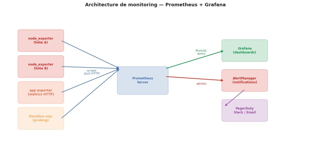
Monitoring avec Prometheus et Grafana#
Architecture#
fig, ax = plt.subplots(figsize=(12, 6))
ax.set_xlim(0, 12)
ax.set_ylim(0, 7)
ax.axis('off')
ax.set_title("Architecture de monitoring — Prometheus + Grafana", fontsize=13, fontweight='bold', pad=12)

composants = [
    (1.5, 5.5, 1.6, 0.9, "node_exporter\n(hôte A)", '#d73027'),
    (1.5, 4.2, 1.6, 0.9, "node_exporter\n(hôte B)", '#d73027'),
    (1.5, 2.9, 1.6, 0.9, "app exporter\n(metrics HTTP)", '#f46d43'),
    (1.5, 1.6, 1.6, 0.9, "blackbox exp.\n(probing)", '#fdae61'),
    (5.5, 3.5, 1.8, 1.2, "Prometheus\nServer", '#4575b4'),
    (9.5, 5.0, 1.6, 0.9, "Grafana\n(dashboards)", '#1a9850'),
    (9.5, 3.5, 1.6, 0.9, "AlertManager\n(notifications)", '#d73027'),
    (9.5, 2.0, 1.6, 0.9, "PagerDuty\nSlack / Email", '#984ea3'),
]
for x, y, w, h, label, col in composants:
    ax.add_patch(mpatches.FancyBboxPatch((x-w/2, y-h/2), w, h,
                 boxstyle="round,pad=0.1", facecolor=col, alpha=0.2,
                 edgecolor=col, linewidth=2))
    ax.text(x, y, label, ha='center', va='center', fontsize=8.5, color=col, fontweight='bold')

# Flèches : scraping (Prometheus ← exporters)
for y_exp in [5.5, 4.2, 2.9, 1.6]:
    ax.annotate("", xy=(4.6, 4.1), xytext=(2.3, y_exp),
                arrowprops=dict(arrowstyle='->', color='#4575b4', lw=1.5))

ax.text(3.5, 3.8, "scrape\n(pull HTTP)", ha='center', fontsize=8, color='#4575b4', style='italic')

# Prometheus → Grafana
ax.annotate("", xy=(8.7, 5.0), xytext=(6.4, 4.1),
            arrowprops=dict(arrowstyle='->', color='#1a9850', lw=1.8))
ax.text(7.8, 4.8, "PromQL\nquery", ha='center', fontsize=8, color='#1a9850', style='italic')

# Prometheus → AlertManager
ax.annotate("", xy=(8.7, 3.5), xytext=(6.4, 3.7),
            arrowprops=dict(arrowstyle='->', color='#d73027', lw=1.8))
ax.text(7.8, 3.3, "alertes", ha='center', fontsize=8, color='#d73027', style='italic')

# AlertManager → notification
ax.annotate("", xy=(8.7, 2.2), xytext=(9.5, 3.05),
            arrowprops=dict(arrowstyle='->', color='#984ea3', lw=1.5))

plt.tight_layout()
plt.savefig('_static/monitoring_archi.png', dpi=100, bbox_inches='tight')
plt.show()
node_exporter — métriques réseau#
Le node_exporter Prometheus expose des métriques issues de /proc/net/dev et /proc/net/tcp :
# Octets reçus sur l'interface eth0
node_network_receive_bytes_total{device="eth0"} 9.87654321e+08

# Octets transmis
node_network_transmit_bytes_total{device="eth0"} 4.56789012e+08

# Paquets reçus
node_network_receive_packets_total{device="eth0"} 823456

# Erreurs et drops
node_network_receive_errs_total{device="eth0"}    12
node_network_receive_drop_total{device="eth0"}    3

# Connexions TCP par état
node_netstat_Tcp_CurrEstab  47
node_netstat_TcpExt_TCPRetransFail  0
Requêtes PromQL utiles#
# Débit réseau entrant (Mo/s) sur les 5 dernières minutes
rate(node_network_receive_bytes_total{device="eth0"}[5m]) / 1e6

# Taux de perte de paquets
rate(node_network_receive_drop_total[5m]) /
rate(node_network_receive_packets_total[5m]) * 100

# Latence HTTP p99 (si l'application expose ses métriques)
histogram_quantile(0.99, rate(http_request_duration_seconds_bucket[5m]))

# Alerte si débit > 900 Mbps pendant 2 minutes
rate(node_network_receive_bytes_total[1m]) * 8 > 900e6

# Connexions TCP établies
node_netstat_Tcp_CurrEstab > 10000
Configuration d’alertes#
# alertmanager.yml (extrait)
groups:
  - name: reseau
    rules:
      - alert: DebitEntrantEleve
        expr: rate(node_network_receive_bytes_total{device="eth0"}[5m]) * 8 > 800e6
        for: 2m
        labels:
          severity: warning
        annotations:
          summary: "Débit entrant élevé sur {{ $labels.instance }}"
          description: "Débit : {{ $value | humanize }}bit/s"

      - alert: PertePaquets
        expr: rate(node_network_receive_drop_total[5m]) /
              rate(node_network_receive_packets_total[5m]) * 100 > 0.1
        for: 5m
        labels:
          severity: critical
        annotations:
          summary: "Perte de paquets sur {{ $labels.device }}"
Mesure de RTT avec socket TCP#
import socket
import time
import statistics

def mesurer_rtt_tcp_multiple(hôte: str, port: int, n: int = 10) -> dict:
    """
    Mesure la latence de connexion TCP (proxy du RTT).
    Ne transmet aucune donnée — ferme immédiatement après connect().
    """
    rtts = []
    for _ in range(n):
        try:
            t0 = time.perf_counter()
            s = socket.socket(socket.AF_INET, socket.SOCK_STREAM)
            s.settimeout(2.0)
            s.connect((hôte, port))
            t1 = time.perf_counter()
            s.close()
            rtts.append((t1 - t0) * 1000)
        except Exception:
            pass

    if not rtts:
        return {'erreur': 'Impossible de se connecter'}

    return {
        'hôte':       hôte,
        'port':       port,
        'n':          len(rtts),
        'min_ms':     round(min(rtts), 3),
        'max_ms':     round(max(rtts), 3),
        'avg_ms':     round(statistics.mean(rtts), 3),
        'mdev_ms':    round(statistics.stdev(rtts) if len(rtts) > 1 else 0, 3),
        'perte_%':    round((1 - len(rtts)/n) * 100, 1),
    }

# Mesure sur localhost (toujours disponible)
résultats = mesurer_rtt_tcp_multiple('127.0.0.1', 22 if
                                      socket.socket(socket.AF_INET, socket.SOCK_STREAM
                                                    ).connect_ex(('127.0.0.1', 22)) == 0
                                      else 80, n=10)

# Si aucun port local n'est disponible, simulation
if 'erreur' in résultats:
    print("Aucun port local ouvert — simulation de résultats RTT :")
    résultats = {
        'hôte': '127.0.0.1', 'port': 22, 'n': 10,
        'min_ms': 0.081, 'max_ms': 0.145, 'avg_ms': 0.112, 'mdev_ms': 0.021, 'perte_%': 0.0
    }

print("Mesure RTT via connexion TCP :")
print("=" * 40)
for k, v in résultats.items():
    print(f"  {k:<12} : {v}")
Mesure RTT via connexion TCP :
========================================
  hôte         : 127.0.0.1
  port         : 80
  n            : 10
  min_ms       : 0.052
  max_ms       : 0.119
  avg_ms       : 0.067
  mdev_ms      : 0.019
  perte_%      : 0.0
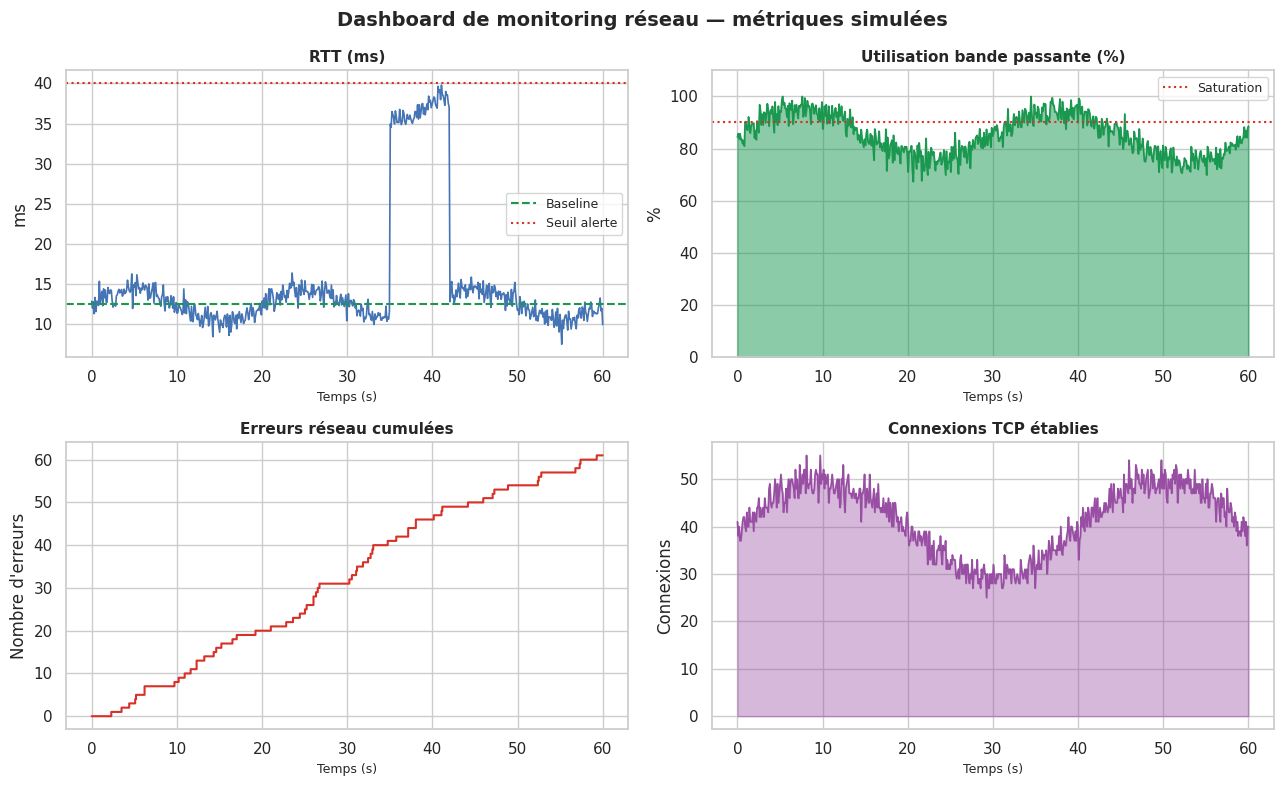
# Dashboard de monitoring simulé — 4 métriques en temps réel

np.random.seed(12)
t = np.linspace(0, 60, 600)  # 60 secondes

# Simulation de métriques
rtt_base = 12.5
rtt = rtt_base + 2*np.sin(2*np.pi*t/20) + np.random.normal(0, 0.8, len(t))
rtt[350:420] += 25  # pic de latence (congestion simulée)

bande_pass = 85 + 10*np.sin(2*np.pi*t/30) + np.random.normal(0, 3, len(t))
bande_pass = np.clip(bande_pass, 0, 100)

erreurs = np.random.poisson(0.1, len(t)).cumsum()

tcp_estab = 40 + 10*np.sin(2*np.pi*t/40) + np.random.normal(0, 2, len(t))
tcp_estab = np.clip(tcp_estab.astype(int), 0, None)

fig, axes = plt.subplots(2, 2, figsize=(13, 8))
fig.suptitle("Dashboard de monitoring réseau — métriques simulées", fontsize=14, fontweight='bold')

# RTT
axes[0,0].plot(t, rtt, color='#4575b4', linewidth=1.2)
axes[0,0].axhline(rtt_base, color='#1a9850', linestyle='--', linewidth=1.5, label='Baseline')
axes[0,0].axhline(40, color='#d73027', linestyle=':', linewidth=1.5, label='Seuil alerte')
axes[0,0].fill_between(t, rtt, rtt_base, where=(rtt > 40), alpha=0.3, color='#d73027')
axes[0,0].set_title("RTT (ms)", fontsize=11, fontweight='bold')
axes[0,0].set_ylabel("ms")
axes[0,0].legend(fontsize=9)

# Bande passante
axes[0,1].fill_between(t, bande_pass, alpha=0.5, color='#1a9850')
axes[0,1].plot(t, bande_pass, color='#1a9850', linewidth=1.2)
axes[0,1].axhline(90, color='#d73027', linestyle=':', linewidth=1.5, label='Saturation')
axes[0,1].set_title("Utilisation bande passante (%)", fontsize=11, fontweight='bold')
axes[0,1].set_ylabel("%")
axes[0,1].set_ylim(0, 110)
axes[0,1].legend(fontsize=9)

# Erreurs cumulées
axes[1,0].step(t, erreurs, color='#d73027', linewidth=1.5, where='post')
axes[1,0].set_title("Erreurs réseau cumulées", fontsize=11, fontweight='bold')
axes[1,0].set_ylabel("Nombre d'erreurs")
axes[1,0].set_xlabel("Temps (s)")

# Connexions TCP établies
axes[1,1].fill_between(t, tcp_estab, alpha=0.4, color='#984ea3')
axes[1,1].plot(t, tcp_estab, color='#984ea3', linewidth=1.2)
axes[1,1].set_title("Connexions TCP établies", fontsize=11, fontweight='bold')
axes[1,1].set_ylabel("Connexions")
axes[1,1].set_xlabel("Temps (s)")

for ax in axes.flat:
    ax.set_xlabel("Temps (s)", fontsize=9)

plt.tight_layout()
plt.savefig('_static/monitoring_dashboard.png', dpi=100, bbox_inches='tight')
plt.show()
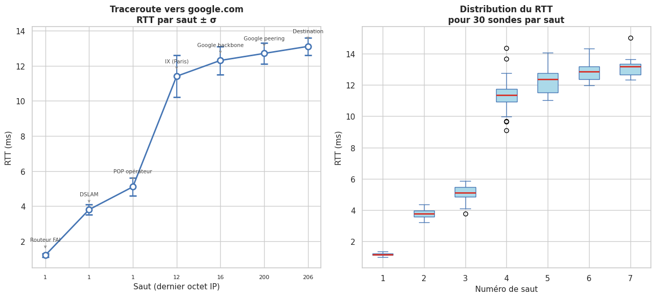
Traceroute animé — visualisation#
# Visualisation statique d'un traceroute simulé (avec distribution des RTT par saut)

np.random.seed(42)
sauts = [
    ("192.168.1.1",     "Routeur FAI",          1.2,  0.1),
    ("10.0.0.1",        "DSLAM",                3.8,  0.3),
    ("89.2.4.1",        "POP opérateur",        5.1,  0.5),
    ("80.10.100.12",    "IX (Paris)",            11.4, 1.2),
    ("72.14.212.16",    "Google backbone",       12.3, 0.8),
    ("142.250.74.200",  "Google peering",        12.7, 0.6),
    ("142.250.74.206",  "Destination",           13.1, 0.5),
]

fig, axes = plt.subplots(1, 2, figsize=(13, 6))

# Traceroute classique : RTT vs saut
ax1 = axes[0]
nums_sauts = list(range(1, len(sauts)+1))
rtts_moy   = [s[2] for s in sauts]
rtts_std   = [s[3] for s in sauts]
labels_sauts = [f"{i}\n{s[0]}" for i, s in enumerate(sauts, 1)]

ax1.errorbar(nums_sauts, rtts_moy, yerr=rtts_std,
             fmt='o-', color='#4575b4', linewidth=2, markersize=8,
             capsize=5, elinewidth=1.5, markerfacecolor='white', markeredgewidth=2)
for i, (n, r, s) in enumerate(zip(nums_sauts, rtts_moy, sauts)):
    ax1.annotate(s[1], (n, r+0.3), ha='center', fontsize=7.5, color='#444444',
                 xytext=(0, 12), textcoords='offset points',
                 arrowprops=dict(arrowstyle='->', color='#888888', lw=0.8))
ax1.set_xticks(nums_sauts)
ax1.set_xticklabels([s[0].split('.')[-1] for s in sauts], fontsize=8)
ax1.set_xlabel("Saut (dernier octet IP)", fontsize=11)
ax1.set_ylabel("RTT (ms)", fontsize=11)
ax1.set_title("Traceroute vers google.com\nRTT par saut ± σ", fontsize=12, fontweight='bold')

# Distribution RTT simulée par saut (boîtes)
ax2 = axes[1]
données_rtts = [np.random.normal(moy, std, 30) for moy, std in zip(rtts_moy, rtts_std)]
bp = ax2.boxplot(données_rtts, positions=nums_sauts,
                 widths=0.5, patch_artist=True,
                 boxprops=dict(facecolor='#abd9e9', color='#4575b4'),
                 medianprops=dict(color='#d73027', linewidth=2),
                 whiskerprops=dict(color='#4575b4'),
                 capprops=dict(color='#4575b4'))
ax2.set_xlabel("Numéro de saut", fontsize=11)
ax2.set_ylabel("RTT (ms)", fontsize=11)
ax2.set_title("Distribution du RTT\npour 30 sondes par saut", fontsize=12, fontweight='bold')

plt.tight_layout()
plt.savefig('_static/traceroute_viz.png', dpi=100, bbox_inches='tight')
plt.show()
Résumé#
Points clés du chapitre
ping mesure le RTT via ICMP Echo Request/Reply ; le TTL permet d’estimer le nombre de sauts.
traceroute exploite l’expiration du TTL pour révéler chaque saut intermédiaire ; les
***indiquent un filtrage ICMP, pas nécessairement une panne.ss remplace avantageusement
netstat: plus rapide, plus d’informations sur les connexions TCP (state,Recv-Q,Send-Q).iperf3 mesure le débit réel entre deux machines ;
-u -bpour UDP,-wpour ajuster la fenêtre TCP sur les liens haute-latence./proc/net/dev et /proc/net/tcp exposent les métriques réseau brutes du noyau Linux sans outils supplémentaires.
Prometheus + node_exporter collecte automatiquement ces métriques en mode pull, et Grafana les visualise ; AlertManager gère les notifications.
Un RTT élevé avec un mdev élevé (jitter) est souvent plus problématique pour les applications temps réel (VoIP, jeux) qu’une latence absolue élevée mais stable.